第4章 连续时间线性时不变系统

4.1 引言

在前一章中，我们识别了系统可能具有的一些性质。其中两个性质是线性和时不变性。本章中，我们将注意力完全集中在同时具备这两个性质的系统上。这样的系统称为线性时不变系统（Linear Time-Invariant，简称 LTI 系统）。

4.2 连续时间卷积

在LTI系统的背景下，一种称为卷积的数学运算显得尤为重要。函数 \(x\) 与 \(h\) 的卷积记作 \(x * h\)，其定义为

\[ \begin{equation*} x * h(t)=\int_{-\infty}^{\infty} x(\tau) h(t-\tau) d \tau \tag{4.1} \end{equation*} \]

这里，星号（即符号“*”）用来表示卷积，而不是乘法。区分卷积与乘法非常重要，因为这两种运算有本质上的不同，通常不会得到相同的结果。

从记号上看，\(x * h\) 表示一个函数，即由 \(x\) 与 \(h\) 卷积而得的函数；而 \(x * h(t)\) 表示在 \(t\) 处对该函数的取值。虽然我们也可以写成 \((x * h)(t)\)，但一般省略这对括号，因为这样不会引起歧义，而且记号更简洁。换句话说，表达式 \(x * h(t)\) 只有一种合理的分组方式，即 \((x * h)(t)\)。而写作 \(x *[h(t)]\) 则是没有意义的，因为卷积需要两个函数作为运算对象，而 \(h(t)\) 是函数 \(h\) 在 \(t\) 处的值，而不是一个函数。因此，\(x * h(t)\) 的唯一合理解释就是 \((x * h)(t)\)。

由于卷积运算在系统理论中被广泛应用，我们需要一种实用的方法来计算卷积积分。假设对于给定的函数 \(x\) 和 \(h\)，我们希望计算

\[ x * h(t)=\int_{-\infty}^{\infty} x(\tau) h(t-\tau) d \tau \]

当然，我们可以“天真”地尝试：对每一个可能的 \(t\) 值单独计算一个积分，从而逐点得到 \(x * h(t)\)。然而，这种方法不可行，因为 \(t\) 可以取无限多个值，因此需要计算无限多个积分。于是我们采用一种稍微不同的方法。我们引入一个中间函数 \(w_{t}\)，定义为

\[ w_{t}(\tau)=x(\tau) h(t-\tau) \]

（注意 \(w_{t}(\tau)\) 是 \(t\) 的隐函数。）这样，我们需要计算的就是

\[ x * h(t)=\int_{-\infty}^{\infty} w_{t}(\tau) d \tau \]

我们注意到，对于大多数实际感兴趣的函数 \(x\) 与 \(h\)，\(w_{t}(\tau)\) 的形式通常在某些 \(t\) 的区间内保持不变。因此，可以通过以下步骤来计算卷积：首先确定 \(w_{t}(\tau)\) 在不同区间内的具体表达式及其有效范围；然后对每个区间分别进行积分。这样，通常只需要计算有限个积分，而不必像之前那样需要无限多个积分。

以上讨论引导我们提出以下计算卷积的一般方法：

1. 将 \(x(\tau)\) 与 \(h(t-\tau)\) 画成关于 \(\tau\) 的函数图像。
2. 起初，考虑一个任意大的负 \(t\)。此时 \(h(t-\tau)\) 将在时间轴上被移到极左侧。
3. 写出 \(w_{t}(\tau)\) 的数学表达式。
4. 逐渐增加 \(t\)，直到 \(w_{t}(\tau)\) 的形式发生变化。记录该表达式有效的区间。
5. 重复步骤3和4，直到 \(t\) 是一个任意大的正值。此时 \(h(t-\tau)\) 被移到时间轴的极右侧。
6. 对于上面得到的每个区间，对 \(w_{t}(\tau)\) 积分，得到 \(x * h(t)\) 在该区间的解析式。
7. 将各个区间的结果拼接起来，从而得到对所有 \(t\) 都成立的卷积结果 \(x * h(t)\)。

例4.1 计算卷积 \(x * h\)，其中

\[ x(t)=\left\{\begin{array}{ll} -1 & -1 \leq t<0 \\ 1 & 0 \leq t<1 \\ 0 & \text { 其他情况 } \end{array} \quad \text { 且 } \quad h(t)=e^{-t} u(t)\right. \]

解：
首先，如图4.1(a)和(b)所示，画出函数 \(x\) 与 \(h\)。接着，确定 \(h\) 的时间反转与时间平移形式。此过程可分两步：
第一步，将 \(h(\tau)\) 时间反转得到 \(h(-\tau)\)，如图4.1(c)；
第二步，将该结果再按 \(t\) 平移，得到 \(h(t-\tau)\)，如图4.1(d)。

此时我们已准备好计算卷积积分。对于每一个可能的 \(t\) 值，我们需要计算 \(x(\tau)\) 与 \(h(t-\tau)\) 的乘积，并对 \(\tau\) 积分。由于 \(x\) 与 \(h\) 的形式较为特殊，可以将问题划分为少数几种情况。这些情况分别由图4.1(e)–(h)表示。

---

第一种情况：\(t<-1\)
由图4.1(e)可见：

\[ \begin{equation*} x * h(t)=\int_{-\infty}^{\infty} x(\tau) h(t-\tau) d \tau=0 \tag{4.2} \end{equation*} \]

---

第二种情况：\(-1 \leq t<0\)
由图4.1(f)可见：

\[ \begin{align*} x * h(t) &=\int_{-\infty}^{\infty} x(\tau) h(t-\tau) d \tau \\ & =\int_{-1}^{t}-e^{\tau-t} d \tau \\ & =-e^{-t} \int_{-1}^{t} e^{\tau} d \tau \\ & =-\left.e^{-t}\left[e^{\tau}\right]\right|_{-1} ^{t} \\ & =-e^{-t}\left[e^{t}-e^{-1}\right] \\ & =e^{-t-1}-1 \tag{4.3} \end{align*} \]

---

第三种情况：\(0 \leq t<1\)
由图4.1(g)可见：

\[ \begin{align*} x * h(t) &=\int_{-\infty}^{\infty} x(\tau) h(t-\tau) d \tau \\ & =\int_{-1}^{0}-e^{\tau-t} d \tau+\int_{0}^{t} e^{\tau-t} d \tau \\ & =-e^{-t} \int_{-1}^{0} e^{\tau} d \tau+e^{-t} \int_{0}^{t} e^{\tau} d \tau \\ & =-\left.e^{-t}\left[e^{\tau}\right]\right|_{-1} ^{0}+\left.e^{-t}\left[e^{\tau}\right]\right|_{0} ^{t} \\ & =-e^{-t}\left[1-e^{-1}\right]+e^{-t}\left[e^{t}-1\right] \\ & =e^{-t}\left[e^{-1}-1+e^{t}-1\right] \\ & =1+\left(e^{-1}-2\right) e^{-t} \tag{4.4} \end{align*} \]

---

第四种情况：\(t \geq 1\)
由图4.1(h)可见：

\[ \begin{align*} x * h(t) &=\int_{-\infty}^{\infty} x(\tau) h(t-\tau) d \tau \\ & =\int_{-1}^{0}-e^{\tau-t} d \tau+\int_{0}^{1} e^{\tau-t} d \tau \\ & =-e^{-t} \int_{-1}^{0} e^{\tau} d \tau+e^{-t} \int_{0}^{1} e^{\tau} d \tau \\ & =-\left.e^{-t}\left[e^{\tau}\right]\right|_{-1} ^{0}+\left.e^{-t}\left[e^{\tau}\right]\right|_{0} ^{1} \\ & =e^{-t}\left[e^{-1}-1+e-1\right] \\ & =\left(e-2+e^{-1}\right) e^{-t} \tag{4.5} \end{align*} \]

---

综合(4.2)、(4.3)、(4.4)与(4.5)的结果：

\[ x * h(t)= \begin{cases} 0 & t<-1 \\ e^{-t-1}-1 & -1 \leq t<0 \\ \left(e^{-1}-2\right) e^{-t}+1 & 0 \leq t<1 \\ \left(e-2+e^{-1}\right) e^{-t} & 1 \leq t \end{cases} \]

卷积结果 \(x * h\) 绘制在图4.1(i)中。

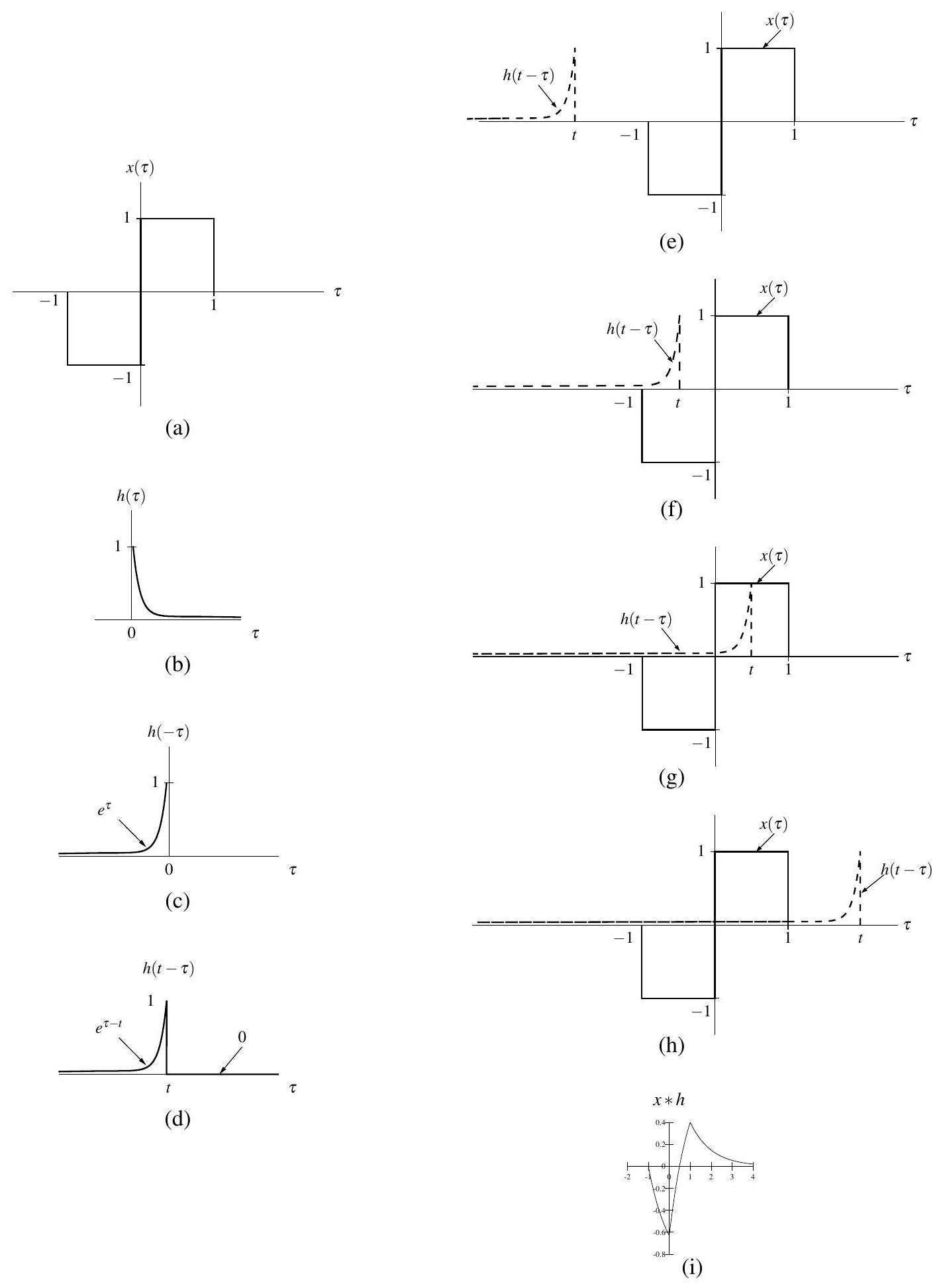
图4.1 卷积 \(x * h\) 的计算过程。(a) 函数 \(x\)；(b) 函数 \(h\)；(c) \(h(-\tau)\) 与 (d) \(h(t-\tau)\) 关于 \(\tau\) 的图像；(e)–(h) 为卷积积分中乘积函数在 \(t<-1\)、\(-1 \leq t<0\)、\(0 \leq t<1\) 和 \(t \geq 1\) 时的情况；(i) 卷积结果 \(x * h\)。

例 4.2 计算卷积 \(x * h\)，其中

\[ x(t)=\left\{\begin{array}{ll} 1 & 0 \leq t<1 \\ 0 & \text { 其他情况 } \end{array} \quad \text { 和 } \quad h(t)= \begin{cases}t & 0 \leq t<1 \\ 0 & \text { 其他情况 }\end{cases}\right. \]

解答。我们首先绘制函数 \(x\) 和 \(h\)，如图 4.2(a) 和 (b) 所示。接下来，我们确定 \(h(\tau)\) 的时间反转及时间平移形式。这可以分两步完成。第一步，将 \(h(\tau)\) 时间反转得到 \(h(-\tau)\)，如图 4.2(c) 所示。第二步，对得到的函数进行时间平移 \(t\)，得到 \(h(t-\tau)\)，如图 4.2(d) 所示。

此时，我们可以开始计算卷积积分。对于每一个可能的 \(t\) 值，我们必须将 \(x(\tau)\) 与 \(h(t-\tau)\) 相乘，并对 \(\tau\) 进行积分。由于 \(x\) 和 \(h\) 的形式，我们可以将这一过程划分为少数几种情况。这些情况对应图 4.2(e) 到 (h) 中所示的情景。

首先，考虑 \(t<0\) 的情况。从图 4.2(e) 可知：

\[ \begin{equation*} x * h(t)=\int_{-\infty}^{\infty} x(\tau) h(t-\tau) d \tau=0 \tag{4.6} \end{equation*} \]

其次，考虑 \(0 \leq t<1\) 的情况。从图 4.2(f) 可知：

\[ \begin{align*} x * h(t)=\int_{-\infty}^{\infty} x(\tau) h(t-\tau) d \tau & =\int_{0}^{t}(t-\tau) d \tau \\ & =\left.\left[t \tau-\frac{1}{2} \tau^{2}\right]\right|_{0} ^{t} \\ & =t^{2}-\frac{1}{2} t^{2} \\ & =\frac{1}{2} t^{2} \tag{4.7} \end{align*} \]

第三，考虑 \(1 \leq t<2\) 的情况。从图 4.2(g) 可知：

\[ \begin{align*} x * h(t)=\int_{-\infty}^{\infty} x(\tau) h(t-\tau) d \tau & =\int_{t-1}^{1}(t-\tau) d \tau \\ & =\left[t \tau-\frac{1}{2} \tau^{2}\right]_{t-1}^{1} \\ & =t-\frac{1}{2}(1)^{2}-\left[t(t-1)-\frac{1}{2}(t-1)^{2}\right] \\ & =t-\frac{1}{2}-\left[t^{2}-t-\frac{1}{2}\left(t^{2}-2 t+1\right)\right] \\ & =-\frac{1}{2} t^{2}+t \tag{4.8} \end{align*} \]

第四，考虑 \(t \geq 2\) 的情况。从图 4.2(h) 可知：

\[ \begin{equation*} x * h(t)=\int_{-\infty}^{\infty} x(\tau) h(t-\tau) d \tau=0 \tag{4.9} \end{equation*} \]

结合 (4.6)、(4.7)、(4.8) 和 (4.9) 的结果，可得：

\[ x * h(t)= \begin{cases}0 & t<0 \\ \frac{1}{2} t^{2} & 0 \leq t<1 \\ -\frac{1}{2} t^{2}+t & 1 \leq t<2 \\ 0 & t \geq 2\end{cases} \]

卷积结果 \(x * h\) 绘制如图 4.2(i)。

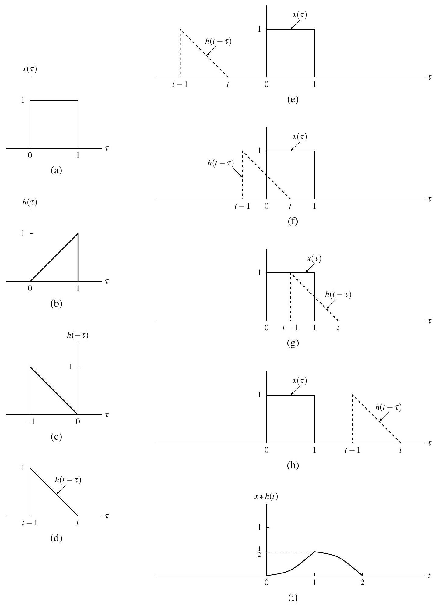
图 4.2：卷积 \(x * h\) 的计算过程。(a) 函数 \(x\)；(b) 函数 \(h\)；(c) \(h(-\tau)\) 与 (d) \(h(t-\tau)\) 关于 \(\tau\) 的图像；卷积积分中乘积函数对应的情况： (e) \(t<0\)，(f) \(0 \leq t<1\)，(g) \(1 \leq t<2\)，(h) \(t \geq 2\)；(i) 卷积结果 \(x * h\)。

例 4.3 计算量 \(x * h\)，其中

\[ x(t)=\left\{\begin{array}{ll} 0 & t<0 \\ t & 0 \leq t<1 \\ -t+2 & 1 \leq t<2 \\ 0 & t \geq 2 \end{array} \text { 和 } h(t)=u(t)-u(t-1)\right. \]

解答。由于 \(x(t)\) 和 \(h(t)\) 的表达式较为复杂，本题可以通过卷积的图形解释来更容易地求解。我们首先绘制函数 \(x\) 和 \(h\)，如图 4.3(a) 和 (b) 所示。

接下来，我们需要确定 \(h(t-\tau)\)，即 \(h(\tau)\) 的时间反转和平移形式。可以分两步完成。第一步，将 \(h(\tau)\) 时间反转得到 \(h(-\tau)\)，如图 4.3(c) 所示。第二步，对得到的信号进行时间平移 \(t\)，得到 \(h(t-\tau)\)，如图 4.3(d) 所示。

此时，我们可以开始计算卷积积分。对于每一个可能的 \(t\) 值，我们必须将 \(x(\tau)\) 与 \(h(t-\tau)\) 相乘，并对 \(\tau\) 积分。根据 \(x\) 和 \(h\) 的形式，可以将这一过程划分为少数几种情况。这些情况对应图 4.3(e) 到 (i) 中所示的情景。

首先，考虑 \(t<0\) 的情况。从图 4.3(e) 可知：

\[ \begin{equation*} x * h(t)=\int_{-\infty}^{\infty} x(\tau) h(t-\tau) d \tau=0 \tag{4.10} \end{equation*} \]

其次，考虑 \(0 \leq t<1\) 的情况。从图 4.3(f) 可知：

\[ \begin{align*} x * h(t)=\int_{-\infty}^{\infty} x(\tau) h(t-\tau) d \tau & =\int_{0}^{t} \tau d \tau \\ & =\left[\frac{1}{2} \tau^{2}\right]_{0}^{t} \\ & =\frac{1}{2} t^{2} \tag{4.11} \end{align*} \]

第三，考虑 \(1 \leq t<2\) 的情况。从图 4.3(g) 可知：

\[ \begin{align*} x * h(t)=\int_{-\infty}^{\infty} x(\tau) h(t-\tau) d \tau & =\int_{t-1}^{1} \tau d \tau+\int_{1}^{t}(-\tau+2) d \tau \\ & =\left[\frac{1}{2} \tau^{2}\right]_{t-1}^{1}+\left[-\frac{1}{2} \tau^{2}+2 \tau\right]_{1}^{t} \\ & =\frac{1}{2}-\left[\frac{1}{2}(t-1)^{2}\right]-\frac{1}{2} t^{2}+2 t-\left[-\frac{1}{2}+2\right] \\ & =-t^{2}+3 t-\frac{3}{2} \tag{4.12} \end{align*} \]

第四，考虑 \(2 \leq t<3\) 的情况。从图 4.3(h) 可知：

\[ \begin{align*} x * h(t)=\int_{-\infty}^{\infty} x(\tau) h(t-\tau) d \tau & =\int_{t-1}^{2}(-\tau+2) d \tau \\ & =\left[-\frac{1}{2} \tau^{2}+2 \tau\right]_{t-1}^{2} \\ & =2-\left[-\frac{1}{2} t^{2}+3 t-\frac{5}{2}\right] \\ & =\frac{1}{2} t^{2}-3 t+\frac{9}{2} \tag{4.13} \end{align*} \]

最后，考虑 \(t \geq 3\) 的情况。从图 4.3(i) 可知：

\[ \begin{equation*} x * h(t)=\int_{-\infty}^{\infty} x(\tau) h(t-\tau) d \tau=0 \tag{4.14} \end{equation*} \]

结合 (4.10)、(4.11)、(4.12)、(4.13) 和 (4.14) 的结果，可得：

\[ x * h(t)= \begin{cases}0 & t<0 \\ \frac{1}{2} t^{2} & 0 \leq t<1 \\ -t^{2}+3 t-\frac{3}{2} & 1 \leq t<2 \\ \frac{1}{2} t^{2}-3 t+\frac{9}{2} & 2 \leq t<3 \\ 0 & t \geq 3\end{cases} \]

卷积结果 \(x * h\) 绘制如图 4.3(j)。

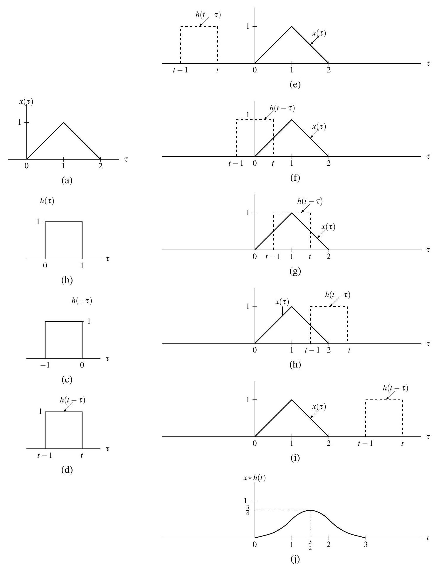
图 4.3：卷积 \(x * h\) 的计算过程。(a) 函数 \(x\)；(b) 函数 \(h\)；(c) \(h(-\tau)\) 与 (d) \(h(t-\tau)\) 关于 \(\tau\) 的图像；卷积积分中乘积函数对应的情况： (e) \(t<0\)，(f) \(0 \leq t<1\)，(g) \(1 \leq t<2\)，(h) \(2 \leq t<3\)，(i) \(t \geq 3\)；(j) 卷积结果 \(x * h\)。

---

例4.4 计算卷积 \(x * h\)，其中

\[ x(t)=e^{-a t} u(t), \quad h(t)=u(t) \]

且 \(a\) 为严格正的实常数。

解： 由于 \(x\) 与 \(h\) 都比较简单，这里我们在不借助图形的情况下求解。本例目标有二：一是展示在足够小心的前提下可以不借助图示直接完成简单卷积；二是说明即便函数较简单，若不借助图示正确地处理也有一定难度，因此画图通常能降低出错概率。

由卷积定义，有

\[ \begin{align*} x * h(t) &=\int_{-\infty}^{\infty} x(\tau) h(t-\tau)\, d \tau \\ &=\int_{-\infty}^{\infty} e^{-a\tau} u(\tau)\, u(t-\tau)\, d \tau \tag{4.15} \end{align*} \]

注意

\[ u(\tau)\,u(t-\tau)= \begin{cases} 1 & 0 \le \tau \text{ 且 } \tau \le t \\ 0 & \text{其他情况} \end{cases} \]

因此被积函数只有在 \(0 \le \tau \le t\) 时才可能非零（这又要求 \(t\ge 0\)）。所以当 \(t<0\) 时，被积函数恒为零，故 \(x * h(t)=0\)。现在考虑 \(t>0\) 的情形，由 (4.15) 得：

\[ \begin{aligned} x * h(t) &=\int_{0}^{t} e^{-a\tau}\, d \tau \\ &=\left[-\frac{1}{a} e^{-a\tau}\right]_{0}^{t} \\ &=\frac{1}{a}\left(1-e^{-a t}\right) \end{aligned} \]

于是得到

\[ \begin{aligned} x * h(t) &=\begin{cases} \frac{1}{a}\left(1-e^{-a t}\right) & t>0 \\ 0 & \text{其他情况} \end{cases} \\ &=\frac{1}{a}\left(1-e^{-a t}\right)u(t) \end{aligned} \]

注意如上所示，不借助图形直接计算卷积在某些步骤上容易出错，即使卷积的函数较为简单。若对某些步骤感到不够清晰，建议画图辅助卷积计算。例如使用如图4.4 所示的图形，通常可以使上述卷积更易于正确计算。

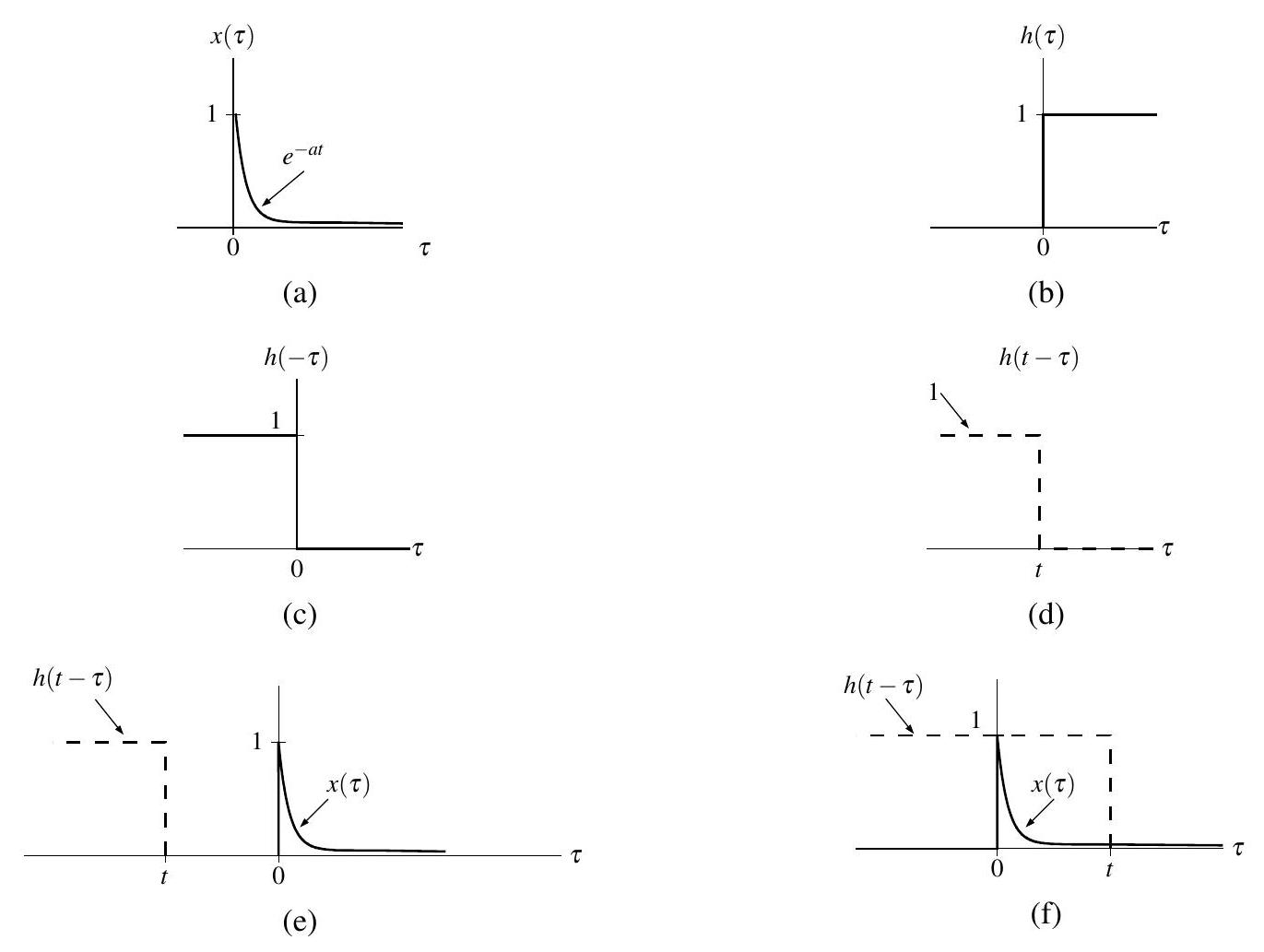
图4.4 卷积 \(x * h\) 的计算过程。(a) 函数 \(x\)；(b) 函数 \(h\)；(c) \(h(-\tau)\) 与 (d) \(h(t-\tau)\) 关于 \(\tau\) 的图像；(e) 与 (f) 分别为卷积积分中乘积函数在 \(t<0\) 与 \(t>0\) 时的情况。

4.3 卷积的性质

由于卷积在研究LTI系统中被频繁使用，因此了解它的一些基本性质是很重要的。下面我们将探讨其中的一些性质。

---

定理4.1（卷积的交换律）
卷积满足交换律。即，对于任意两个函数 \(x\) 和 \(h\)，

\[ \begin{equation*} x * h=h * x \tag{4.16} \end{equation*} \]

换句话说，卷积的结果与其操作数的顺序无关。

证明： 我们来证明上述交换律。首先，展开(4.16)左边：

\[ x * h(t)=\int_{-\infty}^{\infty} x(\tau) h(t-\tau)\, d \tau \]

接下来，进行变量替换。令 \(v=t-\tau\)，则 \(\tau=t-v\)，且 \(d\tau=-dv\)。代入上式得：

\[ \begin{aligned} x * h(t) & =\int_{t+\infty}^{t-\infty} x(t-v) h(v)(-dv) \\ & =\int_{\infty}^{-\infty} x(t-v) h(v)(-dv) \\ & =\int_{-\infty}^{\infty} x(t-v) h(v)\, dv \\ & =\int_{-\infty}^{\infty} h(v) x(t-v)\, dv \\ & =h * x(t) \end{aligned} \]

（注意：我们利用了积分性质 \(\int_{a}^{b} f(x)\, dx=-\int_{b}^{a} f(x)\, dx\)。）因此，卷积满足交换律。

---

定理 4.2（卷积的结合律）。卷积是结合的。也就是说，对于任意三个函数 \(x, h_{1}\) 和 \(h_{2}\)，有

\[ \begin{equation*} \left(x * h_{1}\right) * h_{2}=x *\left(h_{1} * h_{2}\right) \tag{4.17} \end{equation*} \]

换句话说，多重卷积的最终结果与卷积操作的分组方式无关。

证明。首先，根据卷积的定义，将 (4.17) 的左边展开如下：

\[ \begin{aligned} \left(\left[x * h_{1}\right] * h_{2}\right)(t) & =\int_{-\infty}^{\infty}\left[x * h_{1}(v)\right] h_{2}(t-v) d v \\ & =\int_{-\infty}^{\infty}\left(\int_{-\infty}^{\infty} x(\tau) h_{1}(v-\tau) d \tau\right) h_{2}(t-v) d v \end{aligned} \]

现在，我们交换积分顺序，得到

\[ \left(\left[x * h_{1}\right] * h_{2}\right)(t)=\int_{-\infty}^{\infty} \int_{-\infty}^{\infty} x(\tau) h_{1}(v-\tau) h_{2}(t-v) d v d \tau \]

将 \(x(\tau)\) 提到内层积分之外，得到

\[ \left(\left[x * h_{1}\right] * h_{2}\right)(t)=\int_{-\infty}^{\infty} x(\tau) \int_{-\infty}^{\infty} h_{1}(v-\tau) h_{2}(t-v) d v d \tau \]

接下来，进行变量代换。令 \(\lambda = v - \tau\)，则 \(v = \lambda + \tau\)，并且 \(d \lambda = d v\)。利用此变量代换，可以写为

\[ \begin{aligned} \left(\left[x * h_{1}\right] * h_{2}\right)(t) & =\int_{-\infty}^{\infty} x(\tau) \int_{-\infty-\tau}^{\infty-\tau} h_{1}(\lambda) h_{2}(t-\lambda-\tau) d \lambda d \tau \\ & =\int_{-\infty}^{\infty} x(\tau) \int_{-\infty}^{\infty} h_{1}(\lambda) h_{2}(t-\lambda-\tau) d \lambda d \tau \\ & =\int_{-\infty}^{\infty} x(\tau)\left(\int_{-\infty}^{\infty} h_{1}(\lambda) h_{2}([t-\tau]-\lambda) d \lambda\right) d \tau \\ & =\int_{-\infty}^{\infty} x(\tau)\left[h_{1} * h_{2}(t-\tau)\right] d \tau \\ & =\left(x *\left[h_{1} * h_{2}\right]\right)(t) \end{aligned} \]

因此，我们证明了卷积具有结合律。

---

定理4.3（卷积的分配律）
卷积满足分配律。即，对于任意三个函数 \(x, h_{1}, h_{2}\)，

\[ \begin{equation*} x *\left(h_{1}+h_{2}\right)=x * h_{1}+x * h_{2} \tag{4.18} \end{equation*} \]

换句话说，卷积对加法具有分配性。

证明： 该性质证明较为简单。展开(4.18)左边：

\[ \begin{aligned} \left(x *\left[h_{1}+h_{2}\right]\right)(t) &=\int_{-\infty}^{\infty} x(\tau)\left[h_{1}(t-\tau)+h_{2}(t-\tau)\right] d\tau \\ &=\int_{-\infty}^{\infty} x(\tau) h_{1}(t-\tau)\, d\tau + \int_{-\infty}^{\infty} x(\tau) h_{2}(t-\tau)\, d\tau \\ &=x * h_{1}(t)+x * h_{2}(t) \end{aligned} \]

因此，我们已经证明了卷积具有分配律。
对于定义在集合元素上的运算，知道该运算的恒等元通常非常有用。考虑实数上的加法和乘法运算。对于任意实数 \(a\)，有 \(a+0=a\)。由于将 0 加到 \(a\) 上没有影响（即结果仍为 \(a\)），因此我们称 0 为加法恒等元。对于任意实数 \(a\)，有 \(1 \cdot a=a\)。由于将 \(a\) 乘以 1 没有影响（即结果仍为 \(a\)），因此我们称 1 为乘法恒等元。想象一下，如果我们不知道 \(a+0=a\) 或 \(1 \cdot a=a\)，算术将会有多困难。因此，恒等值显然具有根本的重要性。

前面，我们引入了一种称为卷积的新运算。因此，结合上述内容，自然会想知道卷积是否存在恒等元。事实上是存在的，如下定理所示。

---

定理4.4（卷积的单位元）
对于任意函数 \(x\)，

\[ \begin{equation*} x * \delta = x \tag{4.19} \end{equation*} \]

换句话说，\(\delta\) 是卷积的单位元（即任意函数 \(x\) 与 \(\delta\) 卷积后仍为 \(x\)）。

证明： 设 \(x\) 为任意函数。根据卷积定义：

\[ x * \delta(t)=\int_{-\infty}^{\infty} x(\tau)\, \delta(t-\tau)\, d\tau \]

进行变量替换。令 \(\lambda=-\tau\)，则 \(\tau=-\lambda\) 且 \(d\tau=-d\lambda\)。代入得：

\[ \begin{align*} x * \delta(t) &=\int_{-(-\infty)}^{-(\infty)} x(-\lambda)\, \delta(t+\lambda)(-1)\, d\lambda \\ &=\int_{\infty}^{-\infty} x(-\lambda)\, \delta(t+\lambda)(-1)\, d\lambda \\ &=\int_{-\infty}^{\infty} x(-\lambda)\, \delta(\lambda+t)\, d\lambda \tag{4.20} \end{align*} \]

利用 \(\delta\) 的等效性质，上式可写为：

\[ \begin{aligned} x * \delta(t) &=\int_{-\infty}^{\infty} x(-[-t])\, \delta(\lambda+t)\, d\lambda \\ &=\int_{-\infty}^{\infty} x(t)\, \delta(\lambda+t)\, d\lambda \end{aligned} \]

将 \(x(t)\) 提到积分外：

\[ x * \delta(t)=x(t)\int_{-\infty}^{\infty} \delta(\lambda+t)\, d\lambda \]

由于 \(\int_{-\infty}^{\infty} \delta(\lambda)\, d\lambda=1\)，因此 \(\int_{-\infty}^{\infty} \delta(\lambda+t)\, d\lambda=1\)。于是得到：

\[ x * \delta(t)=x(t) \]

因此，\(\delta\) 是卷积的单位元（即 \(x * \delta=x\)）。（或者，也可以直接利用抽样性质对式(4.20)进行处理以得到所需结果。）

4.4 周期卷积

两个周期函数的卷积通常没有良好的定义。这促使我们提出一种适用于周期信号的替代卷积概念，称为周期卷积。两个 \(T\) 周期函数 \(x\) 和 \(h\) 的周期卷积，记作 \(x \circledast h\)，定义为

\[ x \circledast h(t)=\int_{T} x(\tau) h(t-\tau) d \tau \]

其中，\(\int_{T}\) 表示在一个长度为 \(T\) 的区间上积分。周期卷积与 \(T\) 周期函数 \(x\) 和 \(h\) 的（线性）卷积之间的关系为

\[ x \circledast h(t)=x_{0} * h(t) \quad \text{ 其中 } \quad x(t)=\sum_{k=-\infty}^{\infty} x_{0}(t-k T) \]

（即 \(x_{0}(t)\) 在 \(x\) 的一个周期内与 \(x(t)\) 相等，而在其他地方为零）。

4.5 表征LTI系统与卷积

在术语上，系统 \(\mathcal{H}\) 的冲激响应 \(h\) 定义为

\[ h=\mathcal{H} \delta \]

换句话说，系统的冲激响应是当输入为 \(\delta\) 时系统产生的输出。事实证明，LTI 系统在输入、输出和冲激响应之间具有一种非常特殊的关系，如下定理所示。

定理 4.5（LTI系统与卷积）。 具有冲激响应 \(h\) 的 LTI 系统 \(\mathcal{H}\) 满足

\[ \mathcal{H} x=x * h . \]

换句话说，LTI 系统执行的是卷积运算。特别地，系统的输出由输入与冲激响应的卷积给出。

证明。 首先，我们假设 \(\mathcal{H}\) 是 LTI（即 \(\mathcal{H}\) 同时具有线性与时不变性）。利用 \(\delta\) 是卷积单位元这一事实，可以写为

\[ \mathcal{H} x=\mathcal{H}\{x * \boldsymbol{\delta}\} . \]

由卷积的定义，我们有

\[ \mathcal{H} x=\mathfrak{H}\left\{\int_{-\infty}^{\infty} x(\tau) \delta(\cdot-\tau) d \tau\right\} \]

由于 \(\mathcal{H}\) 是线性的，我们可以将积分和 \(x(\tau)\)（它相对于 \(\mathcal{H}\) 的运算来说是常数）提出到 \(\mathcal{H}\) 外，从而得到

\[ \begin{equation*} \mathcal{H} x=\int_{-\infty}^{\infty} x(\tau) \mathcal{H}\{\delta(\cdot-\tau)\} d \tau . \tag{4.21} \end{equation*} \]

由于 \(\mathcal{H}\) 是时不变的，我们可以交换 \(\mathcal{H}\) 与 \(\delta\) 的时间平移顺序，即

\[ \mathcal{H}\{\delta(\cdot-\tau)\}=h(\cdot-\tau) . \]

因此，我们可以将式 (4.21) 改写为

\[ \begin{aligned} \mathcal{H} x & =\int_{-\infty}^{\infty} x(\tau) h(\cdot-\tau) d \tau \\ & =x * h \end{aligned} \]

因此，我们已经证明了 \(\mathcal{H} x=x * h\)，其中 \(h=\mathcal{H} \delta\)。

根据定理 4.5，LTI 系统的行为完全由其冲激响应所表征。也就是说，如果已知系统的冲激响应，我们就能确定系统对任意输入的响应。因此，冲激响应为研究 LTI 系统提供了一个非常有力的工具。

---

例 4.5. 考虑一个冲激响应为

\[ \begin{equation*} h(t)=u(t) \tag{4.22} \end{equation*} \]

的 LTI 系统 \(\mathcal{H}\)。

证明 \(\mathcal{H}\) 可由下式表征：

\[ \begin{equation*} \mathcal{H} x(t)=\int_{-\infty}^{t} x(\tau) d \tau \tag{4.23} \end{equation*} \]

（即，\(\mathcal{H}\) 对应于一个理想积分器）。

解。 由于系统是 LTI 的，我们有

\[ \mathcal{H} x(t)=x * h(t) \]

将 (4.22) 代入上述方程并化简，得到

\[ \begin{aligned} \mathcal{H} x(t) & =x * h(t) \\ & =x * u(t) \\ & =\int_{-\infty}^{\infty} x(\tau) u(t-\tau) d \tau \\ & =\int_{-\infty}^{t} x(\tau) u(t-\tau) d \tau+\int_{t^{+}}^{\infty} x(\tau) u(t-\tau) d \tau \\ & =\int_{-\infty}^{t} x(\tau) d \tau \end{aligned} \]

因此，冲激响应如 (4.22) 给出的系统实际上就是由 (4.23) 给出的理想积分器。

---

例 4.6. 考虑一个 LTI 系统 \(\mathcal{H}\)，其冲激响应 \(h\) 为

\[ h(t)= \begin{cases}1 & 0 \leq t<1 \\ 0 & \text { 其他情况 }\end{cases} \]

求系统对输入

\[ x(t)= \begin{cases}1 & 0 \leq t<1 \\ 0 & \text { 其他情况 }\end{cases} \]

的响应 \(y\)，并作图。

解。 函数 \(x\) 与 \(h\) 的图像分别如图 4.5(a) 与 (b) 所示。由于系统是 LTI 的，我们知道

\[ y(t)=x * h(t) \]

因此，为了求系统对输入 \(x\) 的响应 \(y\)，我们只需要计算卷积 \(x * h\)。

首先如图 4.5(a)、(b) 所示绘制 \(x\) 与 \(h\)。接着，确定 \(h(\tau)\) 的时间反转和平移。这个过程分两步：第一步，将 \(h(\tau)\) 时间反转得到 \(h(-\tau)\)，如图 4.5(c) 所示；第二步，将其再平移 \(t\) 单位，得到 \(h(t-\tau)\)，如图 4.5(d) 所示。

到此为止，我们已经准备好计算卷积积分。对每个可能的 \(t\) 值，都需要将 \(x(\tau)\) 与 \(h(t-\tau)\) 相乘并对 \(\tau\) 积分。由于 \(x\) 与 \(h\) 的形式简单，我们可以将计算分成几个情况。这些情况如图 4.5(e)–(h) 所示。

第一种情况：\(t<0\)。 从图 4.5(e) 可见

\[ \begin{equation*} x * h(t)=\int_{-\infty}^{\infty} x(\tau) h(t-\tau) d \tau=0 \tag{4.24} \end{equation*} \]

第二种情况：\(0 \leq t<1\)。 从图 4.5(f) 可见

\[ \begin{align*} x * h(t)=\int_{-\infty}^{\infty} x(\tau) h(t-\tau) d \tau & =\int_{0}^{t} d \tau \\ & =\left.[\tau]\right|_{0} ^{t} \\ & =t \tag{4.25} \end{align*} \]

第三种情况：\(1 \leq t<2\)。 从图 4.5(g) 可见

\[ \begin{align*} x * h(t)=\int_{-\infty}^{\infty} x(\tau) h(t-\tau) d \tau & =\int_{t-1}^{1} d \tau \\ & =\left.[\tau]\right|_{t-1} ^{1} \\ & =1-(t-1) \\ & =2-t \tag{4.26} \end{align*} \]

第四种情况：\(t \geq 2\)。 从图 4.5(h) 可见

\[ \begin{equation*} x * h(t)=\int_{-\infty}^{\infty} x(\tau) h(t-\tau) d \tau=0 \tag{4.27} \end{equation*} \]

综合 (4.24)、(4.25)、(4.26)、(4.27) 的结果，我们有

\[ x * h(t)= \begin{cases}0 & t<0 \\ t & 0 \leq t<1 \\ 2-t & 1 \leq t<2 \\ 0 & t \geq 2\end{cases} \]

卷积结果 \(x * h\) 如图 4.5(i) 所示。系统对给定输入的响应 \(y\) 就是 \(x * h\)。

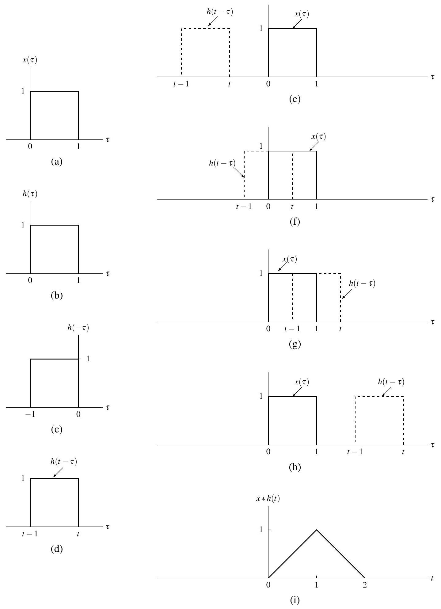
图 4.5： 卷积 \(x * h\) 的计算过程。(a) 函数 \(x\)；(b) 函数 \(h\)；(c) \(h(-\tau)\) 与 (d) \(h(t-\tau)\) 关于 \(\tau\) 的图像；(e) \(t<0\)，(f) \(0 \leq t<1\)，(g) \(1 \leq t<2\)，(h) \(t \geq 2\) 时卷积积分中的乘积对应函数；以及 (i) 卷积结果 \(x * h\)。

4.6 LTI系统的阶跃响应

系统 \(\mathcal{H}\) 的阶跃响应 \(s\) 定义为

\[ s=\mathcal{H} u \]

（即，系统的阶跃响应是其对单位阶跃函数输入所产生的输出）。在 LTI 系统的情形下，阶跃响应与冲激响应之间存在紧密联系，如下定理所示。

定理 4.6. LTI 系统的阶跃响应 \(s\) 与冲激响应 \(h\) 的关系为

\[ h(t)=\frac{d s(t)}{d t} \quad \text { 且 } \quad s(t)=\int_{-\infty}^{t} h(\tau) d \tau \]

也就是说，冲激响应 \(h\) 是阶跃响应 \(s\) 的导数。

证明。 利用 \(s=u * h\) 这一事实，可以写为

\[ \begin{aligned} s(t) & =u * h(t) \\ & =h * u(t) \\ & =\int_{-\infty}^{\infty} h(\tau) u(t-\tau) d \tau \\ & =\int_{-\infty}^{t} h(\tau) d \tau \end{aligned} \]

因此，\(s\) 可以通过对 \(h\) 积分得到。对 \(s\) 求导，得到

\[ \begin{aligned} \frac{d s(t)}{d t} & =\lim _{\Delta t \rightarrow 0} \frac{s(t+\Delta t)-s(t)}{\Delta t} \\ & =\lim _{\Delta t \rightarrow 0} \frac{1}{\Delta t}\left[\int_{-\infty}^{t+\Delta t} h(\tau) d \tau-\int_{-\infty}^{t} h(\tau) d \tau\right] \\ & =\lim _{\Delta t \rightarrow 0} \frac{1}{\Delta t} \int_{t}^{t+\Delta t} h(\tau) d \tau \\ & =\lim _{\Delta t \rightarrow 0} \frac{1}{\Delta t}(h(t) \Delta t) \\ & =h(t) \end{aligned} \]

因此，\(h\) 是 \(s\) 的导数。

阶跃响应在实际应用中常常非常重要，因为它可以用来确定 LTI 系统的冲激响应。特别地，可以通过对阶跃响应求导来得到冲激响应。从实际角度看，阶跃响应更适合通过实验测量来表征系统。显然，我们无法直接测量系统的冲激响应，因为在现实世界中无法产生单位冲激函数或其精确近似。但我们可以在现实中产生较好的单位阶跃函数近似。因此，可以通过测量阶跃响应来推导出冲激响应。

4.7 连续时间LTI系统的方框图表示

在实际应用中，常常将连续时间 LTI 系统用方框图表示会更为方便。由于 LTI 系统完全由其冲激响应表征，因此在方框图中我们通常用系统的冲激响应来标注该系统。也就是说，我们可以将输入为 \(x\)、输出为 \(y\)、冲激响应为 \(h\) 的 LTI 系统表示为图 4.6 所示的形式。

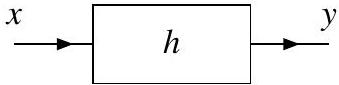
图 4.6： 连续时间 LTI 系统的方框图表示，输入为 \(x\)，输出为 \(y\)，冲激响应为 \(h\)。

4.8 连续时间LTI系统的互连

假设我们有一个输入为 \(x\)、输出为 \(y\)、冲激响应为 \(h\) 的 LTI 系统。我们知道 \(x\) 与 \(y\) 的关系为 \(y=x * h\)。换句话说，该系统可以看作执行卷积运算。利用前面介绍的卷积性质，我们可以推导出系列和并联互连系统的冲激响应之间的一些等效关系。

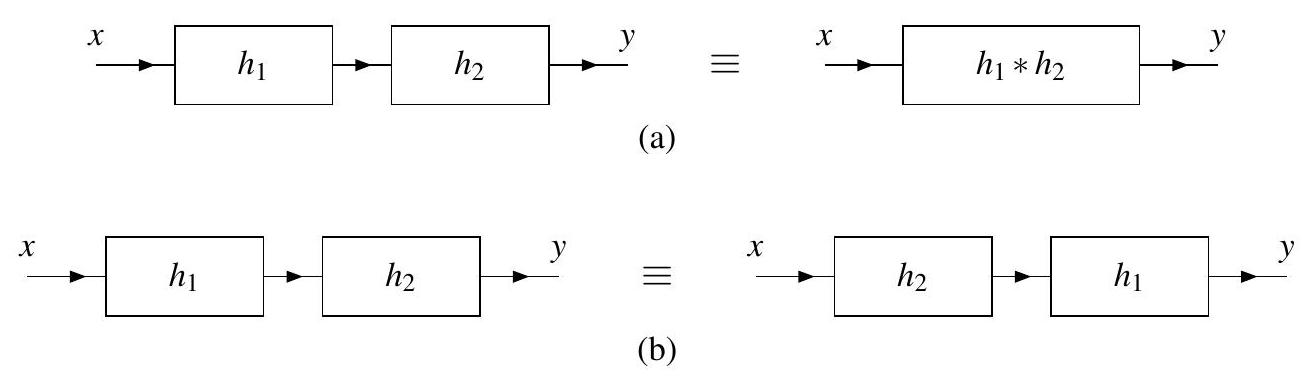
图 4.7： 连续时间 LTI 系统系列互连的等效关系。(a) 第一种等效关系，(b) 第二种等效关系。

考虑两个冲激响应分别为 \(h_{1}\) 和 \(h_{2}\) 的 LTI 系统，它们以串联方式连接，如图 4.7(a) 左侧所示。从图 4.7(a) 左侧的方框图，我们有

\[ y=\left(x * h_{1}\right) * h_{2} . \]

由于卷积的结合律，这等价于

\[ y=x *\left(h_{1} * h_{2}\right) . \]

因此，两个 LTI 系统的串联互连表现为一个冲激响应为 \(h_{1} * h_{2}\) 的单一 LTI 系统。也就是说，如图 4.7(a) 所示的等效关系成立。

考虑两个冲激响应分别为 \(h_{1}\) 和 \(h_{2}\) 的 LTI 系统，它们以串联方式连接，如图 4.7(b) 左侧所示。从图 4.7(b) 左侧的方框图，我们有

\[ y=\left(x * h_{1}\right) * h_{2} . \]

由于卷积具有结合律和交换律，这等价于

\[ \begin{aligned} y & =x *\left(h_{1} * h_{2}\right) \\ & =x *\left(h_{2} * h_{1}\right) \\ & =\left(x * h_{2}\right) * h_{1} . \end{aligned} \]

因此，交换两个 LTI 系统的位置不会改变整体系统的输入输出行为。也就是说，如图 4.7(b) 所示的等效关系成立。

考虑两个冲激响应分别为 \(h_{1}\) 和 \(h_{2}\) 的 LTI 系统，它们以并联方式连接，如图 4.8 左侧所示。从图 4.8 左侧的方框图，我们有

\[ y=x * h_{1}+x * h_{2} . \]

由于卷积具有分配律，该方程可以改写为

\[ y=x *\left(h_{1}+h_{2}\right) . \]

因此，两个 LTI 系统的并联互连表现为一个冲激响应为 \(h_{1}+h_{2}\) 的单一 LTI 系统。也就是说，如图 4.8 所示的等效关系成立。

图 4.8： 连续时间 LTI 系统并联互连的等效关系。

---

例 4.7. 考虑输入为 \(x\)、输出为 \(y\)、冲激响应为 \(h\) 的系统，如图 4.9 所示。方框图中的每个子系统都是 LTI 系统，并标注了其冲激响应。求整体系统的冲激响应 \(h\)。

解： 第一种解法。 从方框图的左半部分，我们可以写出

\[ \begin{aligned} v(t) & =x(t)+x * h_{1}(t)+x * h_{2}(t) \\ & =x * \delta(t)+x * h_{1}(t)+x * h_{2}(t) \\ & =\left(x *\left[\delta+h_{1}+h_{2}\right]\right)(t) \end{aligned} \]

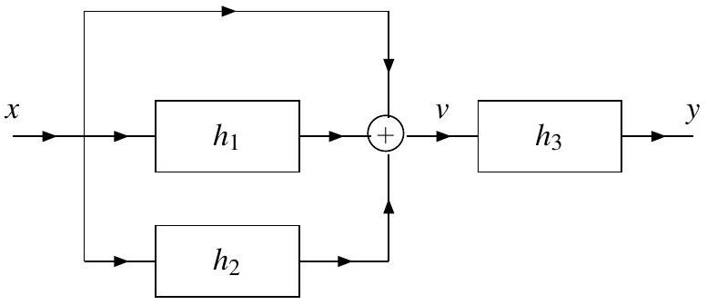
图 4.9： 系统互连示例。

类似地，从方框图的右半部分，我们有

\[ y(t)=v * h_{3}(t) . \]

将 \(v\) 的表达式代入上述方程，得到

\[ \begin{aligned} y(t) & =v * h_{3}(t) \\ & =\left(x *\left[\delta+h_{1}+h_{2}\right]\right) * h_{3}(t) \\ & =x *\left[h_{3}+h_{1} * h_{3}+h_{2} * h_{3}\right](t) . \end{aligned} \]

因此，整体系统的冲激响应 \(h\) 为

\[ h(t)=h_{3}(t)+h_{1} * h_{3}(t)+h_{2} * h_{3}(t) . \]

第二种解法。 设 \(\mathcal{H}, \mathcal{H}_{1}, \mathcal{H}_{2}, \mathcal{H}_{3}\) 分别表示冲激响应为 \(h, h_{1}, h_{2}, h_{3}\) 的系统对应的算子。从给定方框图的左半部分和右半部分，分别有

\[ v=x+\mathcal{H}_{1} x+\mathcal{H}_{2} x \quad \text { 和 } \quad y=\mathcal{H}_{3} v, \]

其中（根据定义）\(y=\mathcal{H} x\)。将这些方程结合，我们得到

\[ \mathcal{H} x=\mathcal{H}_{3}\left(x+\mathcal{H}_{1} x+\mathcal{H}_{2} x\right) . \]

根据冲激响应的定义，\(h=\mathcal{H} \delta, h_{1}=\mathcal{H}_{1} \delta, h_{2}=\mathcal{H}_{2} \delta, h_{3}=\mathcal{H}_{3} \delta\)。因此，我们有

\[ \begin{aligned} h & =\mathcal{H} \delta \\ & =\mathcal{H}_{3}\left(\delta+\mathcal{H}_{1} \delta+\mathcal{H}_{2} \delta\right) . \end{aligned} \]

由于 \(\mathcal{H}_{1}, \mathcal{H}_{2}, \mathcal{H}_{3}\) 是 LTI 系统（意味着 \(\mathcal{H}_{1} x=x * h_{1}, \mathcal{H}_{2} x=x * h_{2}, \mathcal{H}_{3} x=x * h_{3}\)），我们可以将上式改写为

\[ \begin{aligned} h & =\mathcal{H}_{3}\left(\delta+h_{1}+h_{2}\right) \\ & =h_{3} *\left(\delta+h_{1}+h_{2}\right) \\ & =h_{3}+h_{1} * h_{3}+h_{2} * h_{3} . \end{aligned} \]

4.9 连续时间LTI系统的性质

在前一章中，我们介绍了一些系统可能具有的性质（例如，记忆性、因果性、BIBO稳定性以及可逆性）。由于 LTI 系统完全由其冲激响应表征，人们可能会好奇，这些性质与冲激响应之间是否存在联系。下面，我们将探讨其中的一些关系。

4.9.1 记忆性

第一个需要考虑的系统性质是记忆性。

定理 4.7（LTI系统的无记忆性）。 具有冲激响应 \(h\) 的 LTI 系统当且仅当满足下式时无记忆性：

\[ h(t)=0 \text { 对所有 } t \neq 0 . \]

证明： 回忆一下，一个系统是无记忆的，当且仅当其任意时刻的输出 \(y\) 仅依赖于该时刻的输入 \(x\)。假设我们有一个输入为 \(x\)、输出为 \(y\)、冲激响应为 \(h\) 的 LTI 系统。某一时刻 \(t_{0}\) 的输出 \(y\) 为

\[ \begin{aligned} y\left(t_{0}\right) & =x * h\left(t_{0}\right) \\ & =h * x\left(t_{0}\right) \\ & =\int_{-\infty}^{\infty} h(\tau) x\left(t_{0}-\tau\right) d \tau \end{aligned} \]

考虑上述积分。为了使系统无记忆，积分结果只能依赖于 \(x(t)\) 在 \(t=t_{0}\) 时的取值。这只有在满足

\[ h(t)=0 \quad \text { 对所有 } t \neq 0 \]

时才可能成立。

由上定理可知，无记忆 LTI 系统的冲激响应 \(h\) 必须具有如下形式：

\[ \begin{equation*} h(t)=K \delta(t) \tag{4.28} \end{equation*} \]

其中 \(K\) 为复常数。因此，所有无记忆 LTI 系统的输入-输出关系均为

\[ \begin{aligned} y(t) & =x *(K \delta)(t) \\ & =K(x * \delta)(t) \\ & =K x(t) \end{aligned} \]

换句话说，无记忆 LTI 系统必须是理想放大器（即，仅进行幅值缩放的系统）。

---

例 4.8. 考虑冲激响应为

\[ h(t)=e^{-a t} u(t), \]

的 LTI 系统，其中 \(a\) 为实常数。判断该系统是否具有记忆性。

解。 由于 \(h(t) \neq 0\) 对某些 \(t \neq 0\)（例如 \(h(1)=e^{-a} \neq 0\)），该系统具有记忆性。

---

例 4.9. 考虑冲激响应为

\[ h(t)=\delta(t) \]

的 LTI 系统。判断该系统是否具有记忆性。

解： 显然，\(h\) 仅在原点非零。这直接由单位冲激函数 \(\delta\) 的定义可知。因此，该系统无记忆（即不具有记忆性）。

4.9.2 因果性

下一个需要考虑的系统性质是因果性。

定理 4.8（LTI系统的因果性）。 具有冲激响应 \(h\) 的 LTI 系统当且仅当满足下式时为因果系统：

\[ h(t)=0 \text { 对所有 } t<0 . \]

（即，\(h\) 是因果的）。

证明： 回忆一下，一个系统是因果的，当且仅当其任意时刻 \(t_{0}\) 的输出 \(y\) 不依赖于 \(t_{0}\) 之后的输入 \(x\)。假设我们有一个输入为 \(x\)、输出为 \(y\)、冲激响应为 \(h\) 的 LTI 系统。任意时刻 \(t_{0}\) 的输出 \(y\) 为

\[ \begin{align*} y\left(t_{0}\right) & =x * h\left(t_{0}\right) \\ & =\int_{-\infty}^{\infty} x(\tau) h\left(t_{0}-\tau\right) d \tau \\ & =\int_{-\infty}^{t_{0}} x(\tau) h\left(t_{0}-\tau\right) d \tau+\int_{t_{0}^{+}}^{\infty} x(\tau) h\left(t_{0}-\tau\right) d \tau \tag{4.29} \end{align*} \]

为了使式 (4.29) 中的 \(y\left(t_{0}\right)\) 不依赖于 \(t>t_{0}\) 的 \(x(t)\)，必须满足

\[ \begin{equation*} h(t)=0 \quad \text { 对 } t<0 \tag{4.30} \end{equation*} \]

（即，\(h\) 是因果的）。此时，式 (4.29) 可简化为

\[ y\left(t_{0}\right)=\int_{-\infty}^{t_{0}} x(\tau) h\left(t_{0}-\tau\right) d \tau \]

显然，该积分结果不依赖于 \(t>t_{0}\) 的 \(x(t)\)（因为 \(\tau\) 从 \(-\infty\) 到 \(t_{0}\) 变化）。因此，如果 LTI 系统的冲激响应 \(h\) 满足 (4.30)，则系统是因果的。

---

例 4.10. 考虑冲激响应为

\[ h(t)=e^{-a t} u(t) \]

的 LTI 系统，其中 \(a\) 为实常数。判断该系统是否因果。

解。 由于 \(h(t)=0\) 对 \(t<0\)（由 \(h(t)\) 中的 \(u(t)\) 因子可知），因此该系统是因果的。

---

例 4.11. 考虑冲激响应为

\[ h(t)=\delta\left(t+t_{0}\right) \]

的 LTI 系统，其中 \(t_{0}\) 为严格正的实常数。判断该系统是否因果。

解。 根据 \(\delta\) 的定义，可知 \(h(t)=0\)，除非 \(t=-t_{0}\)。由于 \(-t_{0}<0\)，因此该系统不是因果的。

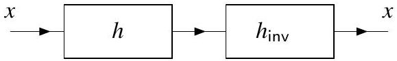
图 4.10： 系统与其逆系统的串联。

4.9.3 可逆性

下一个需要考虑的系统性质是可逆性。
定理 4.9（LTI 系统的逆）。设 \(\mathcal{H}\) 是一个冲激响应为 \(h\) 的 LTI 系统。如果 \(\mathcal{H}\) 的逆 \(\mathcal{H}^{-1}\) 存在，则 \(\mathcal{H}^{-1}\) 也是 LTI 系统，并且具有满足下式的冲激响应 \(h_{\mathrm{inv}}\)：

\[ h * h_{\mathrm{inv}}=\delta . \]

证明：首先，我们需要证明 LTI 系统的逆系统（若存在）也必须是 LTI 系统。然而，这部分证明留作练习题 4.10 给读者完成。（解决该问题的一般方法是：1）如果线性系统的逆存在，则它是线性的；2）如果时不变系统的逆存在，则它是时不变的。）我们假设这部分证明已经完成，并继续进行。

假设逆系统 \(\mathcal{H}^{-1}\) 存在。则有：

\[ \mathcal{H} x = x * h \quad \text{且} \quad \mathcal{H}^{-1} x = x * h_{\mathrm{inv}} . \]

根据逆系统的定义，对于任意函数 \(x\)，有：

\[ \mathcal{H}^{-1} \mathcal{H} x = x . \]

展开前式的左边，我们得到：

\[ \begin{align*} & \mathcal{H}^{-1}[x * h] = x \\ \Leftrightarrow \quad & x * h * h_{\mathrm{inv}} = x . \tag{4.31} \end{align*} \]

该关系在图 4.10 中有图示表示。由于单位冲激函数是卷积恒等元，我们可以等价地将 (4.31) 改写为：

\[ x * h * h_{\mathrm{inv}} = x * \delta . \]

然而，这个方程必须对任意 \(x\) 都成立。因此，通过比较方程两边，我们可以得到：

\[ \begin{equation*} h * h_{\mathrm{inv}} = \delta . \tag{4.32} \end{equation*} \]

因此，如果 \(\mathcal{H}^{-1}\) 存在，则它必须具有满足 (4.32) 的冲激响应 \(h_{\mathrm{inv}}\)。证明完毕。

根据上述定理，我们得到如下结果：

定理 4.10（LTI 系统的可逆性）。冲激响应为 \(h\) 的 LTI 系统 \(\mathcal{H}\) 当且仅当存在函数 \(h_{\mathrm{inv}}\) 满足：

\[ h * h_{\mathrm{inv}} = \delta . \]

证明：该证明可以直接从定理 4.9 的结果得出，只需注意到 \(\mathcal{H}\) 可逆等价于 \(\mathcal{H}^{-1}\) 的存在即可。

例 4.12：考虑冲激响应为

\[ h(t) = A \delta(t - t_0), \]

的 LTI 系统 \(\mathcal{H}\)，其中 \(A\) 和 \(t_0\) 为实常数，且 \(A \neq 0\)。判断 \(\mathcal{H}\) 是否可逆，如果可逆，求出系统 \(\mathcal{H}^{-1}\) 的冲激响应 \(h_{\mathrm{inv}}\)。

解：若系统 \(\mathcal{H}^{-1}\) 存在，其冲激响应 \(h_{\mathrm{inv}}\) 满足方程：

\[ \begin{equation*} h * h_{\mathrm{inv}} = \delta . \tag{4.33} \end{equation*} \]

我们尝试求解 \(h_{\mathrm{inv}}\)。将给定的 \(h\) 代入 (4.33) 并进行简单代数变换，可得：

\[ \begin{aligned} & h * h_{\mathrm{inv}}(t) = \delta(t) \\ \Rightarrow & \int_{-\infty}^{\infty} h(\tau) h_{\mathrm{inv}}(t-\tau) \, d\tau = \delta(t) \\ \Rightarrow & \int_{-\infty}^{\infty} A \delta(\tau - t_0) h_{\mathrm{inv}}(t-\tau) \, d\tau = \delta(t) \\ \Rightarrow & \int_{-\infty}^{\infty} \delta(\tau - t_0) h_{\mathrm{inv}}(t-\tau) \, d\tau = \frac{1}{A} \delta(t) \end{aligned} \]

利用单位冲激函数的筛选性质，可以将上式中的积分简化为：

\[ \begin{align*} & \left. h_{\mathrm{inv}}(t-\tau) \right|_{\tau = t_0} = \frac{1}{A} \delta(t) \\ \Rightarrow \quad & h_{\mathrm{inv}}(t - t_0) = \frac{1}{A} \delta(t) . \tag{4.34} \end{align*} \]

将 \(t + t_0\) 代入上式中的 \(t\)，得到：

\[ \begin{gathered} h_{\mathrm{inv}}([t + t_0] - t_0) = \frac{1}{A} \delta(t + t_0) \quad \Leftrightarrow \\ h_{\mathrm{inv}}(t) = \frac{1}{A} \delta(t + t_0) . \end{gathered} \]

由于 \(A \neq 0\)，函数 \(h_{\mathrm{inv}}\) 始终有定义。因此，\(\mathcal{H}^{-1}\) 存在，故 \(\mathcal{H}\) 可逆。

例 4.13：考虑图 4.11 所示的系统，其输入为 \(x\)，输出为 \(y\)。方框图中的每个子系统都是 LTI 系统，并标注了其冲激响应。利用逆系统的概念，将 \(y\) 用 \(x\) 表示出来。

图 4.11：具有输入 \(x\) 和输出 \(y\) 的反馈系统。

解：由图 4.11 可得：

\[ \begin{gather*} v = x - y * h_2 \quad \text{且} \tag{4.35} \\ y = v * h_1 . \tag{4.36} \end{gather*} \]

将 (4.35) 代入 (4.36) 并进行化简，得到：

\[ \begin{align*} & y = \left[x - y * h_2\right] * h_1 \\ \Rightarrow & y = x * h_1 - y * h_2 * h_1 \\ \Rightarrow & y + y * h_2 * h_1 = x * h_1 \\ \Rightarrow & y * \delta + y * h_2 * h_1 = x * h_1 \\ \Rightarrow & y * \left[\delta + h_2 * h_1\right] = x * h_1 . \tag{4.37} \end{align*} \]

为方便起见，我们现在定义函数 \(g\) 为：

\[ \begin{equation*} g = \delta + h_2 * h_1 \tag{4.38} \end{equation*} \]

于是，可以将 (4.37) 改写为：

\[ \begin{equation*} y * g = x * h_1 . \tag{4.39} \end{equation*} \]

到此，我们几乎已经得出了 \(y\) 关于 \(x\) 的表达式。为了完成求解，需要将方程左侧的 \(g\) 消去。为此，我们使用逆系统的概念。考虑冲激响应为 \(g\) 的系统的逆系统，该逆系统的冲激响应为 \(g_{\mathrm{inv}}\)，满足：

\[ \begin{equation*} g * g_{\mathrm{inv}} = \delta \tag{4.40} \end{equation*} \]

该关系由逆系统的定义得出。现在，我们利用 \(g_{\mathrm{inv}}\) 来简化 (4.39)，得到：

\[ \begin{aligned} & y * g = x * h_1 \\ \Rightarrow & y * g * g_{\mathrm{inv}} = x * h_1 * g_{\mathrm{inv}} \\ \Rightarrow & y * \delta = x * h_1 * g_{\mathrm{inv}} \\ \Rightarrow & y = x * h_1 * g_{\mathrm{inv}} \end{aligned} \]

因此，输出 \(y\) 可以用输入 \(x\) 表示为：

\[ y = x * h_1 * g_{\mathrm{inv}} \]

其中，\(g_{\mathrm{inv}}\) 由 (4.40) 给出，\(g\) 由 (4.38) 给出。

4.9.4 BIBO 稳定性

最后需要考虑的系统性质是 BIBO 稳定性。
定理 4.11（LTI 系统的 BIBO 稳定性）。设 LTI 系统的冲激响应为函数 \(h\)，则该系统当且仅当满足下式时是 BIBO 稳定的：

\[ \begin{equation*} \int_{-\infty}^{\infty} |h(t)| \, dt < \infty \tag{4.41} \end{equation*} \]

（即 \(h\) 是绝对可积的）。

严格来说，该定理要求 \(h\) 为勒贝格可测且局部可积 [17]。因此，例如当 \(h = \delta\) 时，该定理并不适用（因为 \(\delta\) 在勒贝格意义下不可测）。然而，这个说明被列为脚注，因为测度论等内容超出了本书的范围。

证明：回想系统的 BIBO 稳定性定义：对于每一个有界输入，系统必须产生有界输出。设有一个 LTI 系统，其输入为 \(x\)，输出为 \(y\)，冲激响应为 \(h\)。

首先，考虑 (4.41) 对 BIBO 稳定性的充分性。假设 \(|x(t)| \le A < \infty\) 对所有 \(t\) 成立（即 \(x\) 有界）。则可以写作：

\[ \begin{aligned} y(t) & = x * h(t) \\ & = h * x(t) \\ & = \int_{-\infty}^{\infty} h(\tau) \, x(t-\tau) \, d\tau \end{aligned} \]

对上式两边取绝对值，可得：

\[ \begin{equation*} |y(t)| = \left| \int_{-\infty}^{\infty} h(\tau) x(t-\tau) \, d\tau \right| \tag{4.42} \end{equation*} \]

可以证明，对于任意两个函数 \(f_1\) 和 \(f_2\)，有：

\[ \left| \int_{-\infty}^{\infty} f_1(t) f_2(t) \, dt \right| \le \int_{-\infty}^{\infty} |f_1(t) f_2(t)| \, dt \]

利用这个不等式，我们可以将 (4.42) 改写为：

\[ |y(t)| \le \int_{-\infty}^{\infty} |h(\tau) x(t-\tau)| \, d\tau = \int_{-\infty}^{\infty} |h(\tau)| |x(t-\tau)| \, d\tau \]

根据假设，\(|x(t)| \le A\) 对所有 \(t\) 成立，因此可以用其上界 \(A\) 替换上式中的 \(|x(t-\tau)|\)，得到：

\[ \begin{equation*} |y(t)| \le \int_{-\infty}^{\infty} |h(\tau)| |x(t-\tau)| \, d\tau \le \int_{-\infty}^{\infty} A |h(\tau)| \, d\tau = A \int_{-\infty}^{\infty} |h(\tau)| \, d\tau \tag{4.43} \end{equation*} \]

因此，有：

\[ \begin{equation*} |y(t)| \le A \int_{-\infty}^{\infty} |h(\tau)| \, d\tau \tag{4.44} \end{equation*} \]

由于 \(A\) 是有限的，由 (4.44) 可知，如果

\[ \begin{equation*} \int_{-\infty}^{\infty} |h(t)| \, dt < \infty \tag{4.45} \end{equation*} \]

（即 \(h\) 是绝对可积的），则输出 \(y\) 有界。因此，冲激响应 \(h\) 的绝对可积性是 BIBO 稳定性的充分条件。

现在，考虑 (4.41) 对 BIBO 稳定性的必要性。假设 \(h\) 不绝对可积，即：

\[ \int_{-\infty}^{\infty} |h(t)| \, dt = \infty \]

在这种情况下，可以证明系统不具有 BIBO 稳定性。首先，考虑如下特定输入：

\[ x(t) = e^{-j \arg[h(-t)]} \]

由于对任意实数 \(\theta\) 有 \(\left| e^{j\theta} \right| = 1\)，因此 \(x\) 有界（即 \(|x(t)| \le 1\) 对所有 \(t\) 成立）。输出 \(y\) 为：

\[ \begin{align*} y(t) & = x * h(t) \\ & = \int_{-\infty}^{\infty} x(\tau) h(t-\tau) \, d\tau \\ & = \int_{-\infty}^{\infty} e^{-j \arg[h(-\tau)]} h(t-\tau) \, d\tau \tag{4.46} \end{align*} \]

考虑 \(t=0\) 时的输出 \(y(0)\)，由 (4.46) 得：

\[ \begin{equation*} y(0) = \int_{-\infty}^{\infty} e^{-j \arg[h(-\tau)]} h(-\tau) \, d\tau \tag{4.47} \end{equation*} \]

由于对任意复数 \(z\) 有 \(e^{-j \arg z} z = |z|\)，因此 \(e^{-j \arg[h(-\tau)]} h(-\tau) = |h(-\tau)|\)，从而 (4.47) 简化为：

\[ \begin{aligned} y(0) & = \int_{-\infty}^{\infty} |h(-\tau)| \, d\tau \\ & = \int_{-\infty}^{\infty} |h(\tau)| \, d\tau \\ & = \infty \end{aligned} \]

因此，有限输入 \(x\) 会产生无界输出 \(y\)（在 \(t=0\) 时 \(y(t)\) 无界）。由此可见，冲激响应 \(h\) 的绝对可积性也是 BIBO 稳定性的必要条件。证明完毕。

例 4.14：考虑冲激响应为

\[ h(t) = e^{a t} u(t) \]

的 LTI 系统，其中 \(a\) 为实常数。确定该系统在何种 \(a\) 值下是 BIBO 稳定的。

解：需要确定何时冲激响应 \(h\) 绝对可积。我们有：

\[ \begin{aligned} \int_{-\infty}^{\infty} |h(t)| \, dt & = \int_{-\infty}^{\infty} |e^{a t} u(t)| \, dt \\ & = \int_{-\infty}^{0} 0 \, dt + \int_{0}^{\infty} e^{a t} \, dt \\ & = \int_{0}^{\infty} e^{a t} \, dt \\ & = \begin{cases} \int_{0}^{\infty} e^{a t} \, dt & a \neq 0 \\ \int_{0}^{\infty} 1 \, dt & a = 0 \end{cases} \\ & = \begin{cases} \left. \frac{1}{a} e^{a t} \right|_0^{\infty} & a \neq 0 \\ \left. t \right|_0^{\infty} & a = 0 \end{cases} \end{aligned} \]

对于 \(a \neq 0\) 的情况：

\[ \begin{aligned} \int_{-\infty}^{\infty} |h(t)| \, dt & = \left. \frac{1}{a} e^{a t} \right|_0^{\infty} \\ & = \frac{1}{a} (e^{a \infty} - 1) \end{aligned} \]

可见，当 \(a<0\) 时积分结果有限，当 \(a>0\) 时积分发散。特别地，当 \(a<0\) 时：

\[ \begin{aligned} \int_{-\infty}^{\infty} |h(t)| \, dt & = 0 - \frac{1}{a} \\ & = -\frac{1}{a} \end{aligned} \]

当 \(a = 0\) 时：

\[ \begin{aligned} \int_{-\infty}^{\infty} |h(t)| \, dt & = \left. t \right|_0^{\infty} \\ & = \infty \end{aligned} \]

因此，有：

\[ \int_{-\infty}^{\infty} |h(t)| \, dt = \begin{cases} -\frac{1}{a} & a < 0 \\ \infty & a \ge 0 \end{cases} \]

换言之，当且仅当 \(a < 0\) 时，冲激响应 \(h\) 绝对可积。由此，系统当且仅当 \(a < 0\) 时 BIBO 稳定。

例 4.15：考虑输入 \(x\) 和输出 \(y\) 为

\[ y(t) = \int_{-\infty}^{t} x(\tau) \, d\tau \]

的 LTI 系统（即理想积分器）。判断该系统是否 BIBO 稳定。

解：首先，求系统的冲激响应 \(h\)：

\[ \begin{aligned} h(t) & = \int_{-\infty}^{t} \delta(\tau) \, d\tau \\ & = \begin{cases} 1 & t \ge 0 \\ 0 & t < 0 \end{cases} \\ & = u(t) \end{aligned} \]

利用此 \(h\)，检查其是否绝对可积：

\[ \begin{aligned} \int_{-\infty}^{\infty} |h(t)| \, dt & = \int_{-\infty}^{\infty} |u(t)| \, dt \\ & = \int_{0}^{\infty} 1 \, dt \\ & = \infty \end{aligned} \]

因此，\(h\) 不绝对可积，系统不 BIBO 稳定。

4.10 连续时间 LTI 系统的特征函数

在第 3.8.7 节中，我们已经介绍了系统特征函数的概念。由于特征函数有可能简化系统相关的数学运算，因此自然会想知道 LTI 系统可能具有哪些特征函数。在这方面，下面的定理非常具有启发性。

定理 4.12（LTI 系统的特征函数）。设任意 LTI 系统 \(\mathcal{H}\) 的冲激响应为 \(h\)，若输入函数为 \(x(t) = e^{s t}\)，其中 \(s\) 为任意复常数（即 \(x\) 为任意复指数函数），则有：

\[ \begin{equation*} \mathcal{H} x(t) = H(s) e^{s t} \tag{4.48a} \end{equation*} \]

其中

\[ \begin{equation*} H(s) = \int_{-\infty}^{\infty} h(\tau) e^{-s \tau} \, d\tau \tag{4.48b} \end{equation*} \]

也就是说，\(x\) 是 \(\mathcal{H}\) 的特征函数，对应的特征值为 \(H(s)\)。注意，(4.48a) 仅对 \(H(s)\) 收敛的 \(s\) 值成立（即 \(s\) 在 \(H\) 的收敛域内）。

证明：首先，观察到系统 \(\mathcal{H}\) 是 LTI 系统当且仅当它执行卷积（即 \(\mathcal{H} x = x * h\) 对某个 \(h\) 成立）。于是有：

\[ \begin{aligned} \mathcal{H} x(t) & = x * h(t) \\ & = h * x(t) \\ & = \int_{-\infty}^{\infty} h(\tau) x(t-\tau) \, d\tau \\ & = \int_{-\infty}^{\infty} h(\tau) e^{s(t-\tau)} \, d\tau \\ & = e^{s t} \int_{-\infty}^{\infty} h(\tau) e^{-s \tau} \, d\tau \\ & = H(s) e^{s t} \end{aligned} \]

术语说明：定理中出现的函数 \(H\)（即定理 4.12 中的 \(H\)）称为系统函数（或传递函数），它完全描述了 LTI 系统的行为。因此，在处理 LTI 系统时，系统函数通常非常有用。事实上，(4.48b) 中出现的积分形式非常重要，它定义了所谓的拉普拉斯变换。我们将在第 7 章深入学习拉普拉斯变换。

需要注意的是，LTI 系统可以具有除复指数函数以外的特征函数。例如，例 3.43 中的系统是 LTI 系统，并且每个函数都是其特征函数。此外，拥有每个复指数函数作为特征函数的系统不一定是 LTI 系统，下面的例子即可说明。

例 4.16。设 \(S\) 为所有复指数函数的集合（即 \(S\) 是所有形如 \(x(t) = a e^{s t}\) 的函数的集合，其中 \(a, s \in \mathbb{C}\)）。考虑系统 \(\mathcal{H}\) 定义为：

\[ \mathcal{H} x = \begin{cases} x & x \in S \\ 1 & \text{否则} \end{cases} \]

对于任意 \(x \in S\)，有 \(\mathcal{H} x = x\)，意味着 \(x\) 是 \(\mathcal{H}\) 的特征函数，特征值为 1。因此，每个复指数函数都是 \(\mathcal{H}\) 的特征函数。

现在证明 \(\mathcal{H}\) 非线性。设 \(a\) 为任意复常数，考虑函数 \(x(t) = t\)。显然，\(x \notin S\)，因此 \(\mathcal{H} x = 1\)，得到：

\[ a \mathcal{H} x = a \]

再考虑函数 \(a x(t) = a t\)，由于 \(a x \notin S\)，有：

\[ \mathcal{H}(a x) = 1 \]

由上式可见，\(\mathcal{H}(a x) = a \mathcal{H} x\) 仅在 \(a=1\) 时成立。因此，\(\mathcal{H}\) 不满足齐次性，因而非线性。因此，\(\mathcal{H}\) 是一个例子，它的每个复指数函数都是特征函数，但该系统并非 LTI 系统。

下面考虑特征函数的应用。由于卷积运算在实际中常常较为繁琐，我们可以利用特征函数在某些情况下避免直接处理卷积。

设有 LTI 系统 \(\mathcal{H}\)，输入 \(x\)，输出 \(y\)，冲激响应 \(h\)，系统函数 \(H\)。假设可以将任意输入信号 \(x\) 表示为复指数的线性组合：

\[ x(t) = \sum_k a_k e^{s_k t} \]

（实际上，许多函数都可以这样表示）。根据 LTI 系统的特征函数性质，系统对输入 \(a_k e^{s_k t}\) 的响应为 \(a_k H(s_k) e^{s_k t}\)。利用此性质以及叠加原理，可得：

\[ \begin{aligned} y(t) & = \mathcal{H} x(t) \\ & = \mathcal{H} \left\{ \sum_k a_k e^{s_k t} \right\}(t) \\ & = \sum_k a_k \mathcal{H} \left\{ e^{s_k t} \right\}(t) \\ & = \sum_k a_k H(s_k) e^{s_k t} \end{aligned} \]

因此，有：

\[ \begin{equation*} y(t) = \sum_k a_k H(s_k) e^{s_k t} \tag{4.49} \end{equation*} \]

由此可见，如果 LTI 系统的输入可以表示为复指数的线性组合，则输出也可以表示为相同复指数的线性组合。此外，注意输入 \(x(t) = \sum_k a_k e^{s_k t}\) 与输出 \(y\) 之间的关系 (4.49) 并未涉及卷积（如 \(y = x * h\)）。实际上，输出公式与输入公式相同，只是在每个复指数项前乘以常数因子 \(H(s_k)\)。实际上，我们利用特征函数将卷积运算简化为乘以常数的操作。

例 4.17：考虑 LTI 系统 \(\mathcal{H}\)，其冲激响应为

\[ h(t) = \delta(t-1) \]

(a) 求系统函数 \(H\)。
(b) 利用系统函数 \(H\) 求系统 \(\mathcal{H}\) 对输入

\[ x(t) = e^t \cos(\pi t) \]

的输出 \(y\)。

解：

(a) 利用 (4.48b) 求系统函数 \(H\)。将给定的 \(h\) 代入 (4.48b) 得：

\[ \begin{aligned} H(s) & = \int_{-\infty}^{\infty} h(t) e^{-s t} \, dt \\ & = \int_{-\infty}^{\infty} \delta(t-1) e^{-s t} \, dt \\ & = \left. e^{-s t} \right|_{t=1} \\ & = e^{-s} \end{aligned} \]

(b) 将输入 \(x\) 重写为复指数形式：

\[ \begin{aligned} x(t) & = e^t \cos(\pi t) \\ & = e^t \left[ \frac{1}{2} (e^{j \pi t} + e^{-j \pi t}) \right] \\ & = \frac{1}{2} e^{(1 + j \pi) t} + \frac{1}{2} e^{(1 - j \pi) t} \end{aligned} \]

因此输入 \(x\) 可表示为

\[ x(t) = \sum_{k=0}^{1} a_k e^{s_k t} \]

其中

\[ a_k = \frac{1}{2} \quad \text{对 } k \in \{0,1\}, \quad s_k = \begin{cases} 1 + j \pi & k = 0 \\ 1 - j \pi & k = 1 \end{cases} \]

利用系统函数 \(H\) 及 LTI 系统的特征函数性质求输出 \(y\)：

\[ \begin{aligned} y(t) & =\sum_{k=0}^1 a_k H\left(s_k\right) e^{s_k t} \\ & =a_0 H\left(s_0\right) e^{s_0 t}+a_1 H\left(s_1\right) e^{s_1 t} \\ & =\frac{1}{2} H(1+j \pi) e^{(1+j \pi) t}+\frac{1}{2} H(1-j \pi) e^{(1-j \pi) t} \\ & =\frac{1}{2} e^{-(1+j \pi)} e^{(1+j \pi) t}+\frac{1}{2} e^{-(1-j \pi)} e^{(1-j \pi) t} \\ & =\frac{1}{2} e^{t-1+j \pi t-j \pi}+\frac{1}{2} e^{t-1-j \pi t+j \pi} \\ & =\frac{1}{2} e^{t-1} e^{j \pi(t-1)}+\frac{1}{2} e^{t-1} e^{-j \pi(t-1)} \\ & =e^{t-1}\left[\frac{1}{2}\left(e^{j \pi(t-1)}+e^{-j \pi(t-1)}\right)\right] \\ & =e^{t-1} \cos [\pi(t-1)] . \end{aligned} \]

可以看到，输出 \(y\) 仅是输入 \(x\) 向右平移 1 个单位时间的结果。这并非巧合，因为具有系统函数 \(H(s) = e^{-s}\) 的 LTI 系统正是理想的单位延迟系统（即实现时间平移 1 的系统）。

4.11 习题

4.11.1 无答案习题

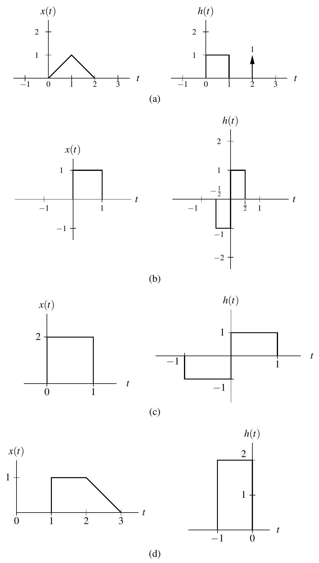
4.1 使用图示法，对于下列图中给出的每对函数 \(x\) 和 \(h\)，直接计算 \(x * h\)。（不要通过计算 \(h * x\) 再利用卷积的交换律间接求 \(x * h\)。）

4.2 对于下列每对函数 \(x\) 和 \(h\)，计算 \(x * h\)。
(a) \(x(t)=e^{a t} u(-t)\) 且 \(h(t)=e^{-a t} u(t)\)，其中 \(a\) 为严格正实常数；
(b) \(x(t)=e^{-j \omega_{0} t} u(t)\) 且 \(h(t)=e^{j \omega_{0} t} u(t)\)，其中 \(\omega_{0}\) 为严格正实常数；
(c) \(x(t)=u(t-2)\) 且 \(h(t)=u(t+3)\)；
(d) \(x(t)=u(t)\) 且 \(h(t)=e^{-2 t} u(t-1)\)；
(e) \(x(t)=u(t-1)-u(t-2)\) 且 \(h(t)=e^{t} u(-t)\)。

4.3 使用图示法，计算下列每对函数 \(x\) 和 \(h\) 的卷积 \(x * h\)。
(a) \(x(t)=e^{t} u(-t)\) 且 \(h(t)= \begin{cases}t-1 & 1 \leq t<2 \\ 0 & \text { 其他情况 }\end{cases}\)
(b) \(x(t)=e^{-|t|}\) 且 \(h(t)=\operatorname{rect}\left(\frac{1}{3}\left[t-\frac{1}{2}\right]\right)\)；
(c) \(x(t)=e^{-t} u(t)\) 且 \(h(t)= \begin{cases}t-1 & 1 \leq t<2 \\ 0 & \text { 其他情况 }\end{cases}\)
(d) \(x(t)=\operatorname{rect}\left(\frac{1}{2} t\right)\) 且 \(h(t)=e^{2-t} u(t-2)\)；
(e) \(x(t)=e^{-|t|}\) 且 \(h(t)= \begin{cases}t+2 & -2 \leq t<-1 \\ 0 & \text { 其他情况 }\end{cases}\)
(f) \(x(t)=e^{-|t|}\) 且 \(h(t)= \begin{cases}t-1 & 1 \leq t<2 \\ 0 & \text { 其他情况 }\end{cases}\)
(g) \(x(t)=\left\{\begin{array}{ll}1-\frac{1}{4} t & 0 \leq t<4 \\ 0 & \text { 其他情况 }\end{array}\right.\) 且 \(h(t)= \begin{cases}t-1 & 1 \leq t<2 \\ 0 & \text { 其他情况 }\end{cases}\)
(h) \(x(t)=\operatorname{rect}\left(\frac{1}{4} t\right)\) 且 \(h(t)=\left\{\begin{array}{ll}2-t & 1 \leq t<2 \\ 0 & \text { 其他情况 }\end{array}\right.\)
(i) \(x(t)=e^{-t} u(t)\) 且 \(h(t)= \begin{cases}t-2 & 2 \leq t<4 \\ 0 & \text { 其他情况 }\end{cases}\)

4.4 证明，对于任意函数 \(x\)，有 \(x * v(t)=x\left(t-t_{0}\right)\)，其中 \(v(t)=\delta\left(t-t_{0}\right)\)，且 \(t_{0}\) 为任意实常数。

4.5 设 \(x, y, h, v\) 为函数，满足 \(y=x * h\) 且

\[ v(t)=\int_{-\infty}^{\infty} x(-\tau-b) h(\tau+a t) d \tau \]

其中 \(a\) 和 \(b\) 为实常数。将 \(v\) 用 \(y\) 表示。

4.6 考虑卷积 \(y=x * h\)。假设卷积 \(y\) 存在，证明下列结论均成立：
(a) 如果 \(x\) 是周期函数，则 \(y\) 是周期函数；
(b) 如果 \(x\) 是偶函数且 \(h\) 是奇函数，则 \(y\) 是奇函数。

4.7 从卷积定义出发，证明如果 \(y=x * h\)，则 \(\mathcal{D} y(t)=[x *(\mathcal{D} h)](t)\)，其中 \(\mathcal{D}\) 表示求导算子。

4.8 设 \(x\) 和 \(h\) 为有限时长函数，满足

\[ x(t)=0 \quad \text { 当 } t<A_{1} \text { 或 } t>A_{2} \quad \text { 且 } \quad h(t)=0 \quad \text { 当 } t<B_{1} \text { 或 } t>B_{2}, \]

其中 \(A_{1}<A_{2}\) 且 \(B_{1}<B_{2}\)。确定 \(x * h(t)\) 必为零的 \(t\) 值范围。

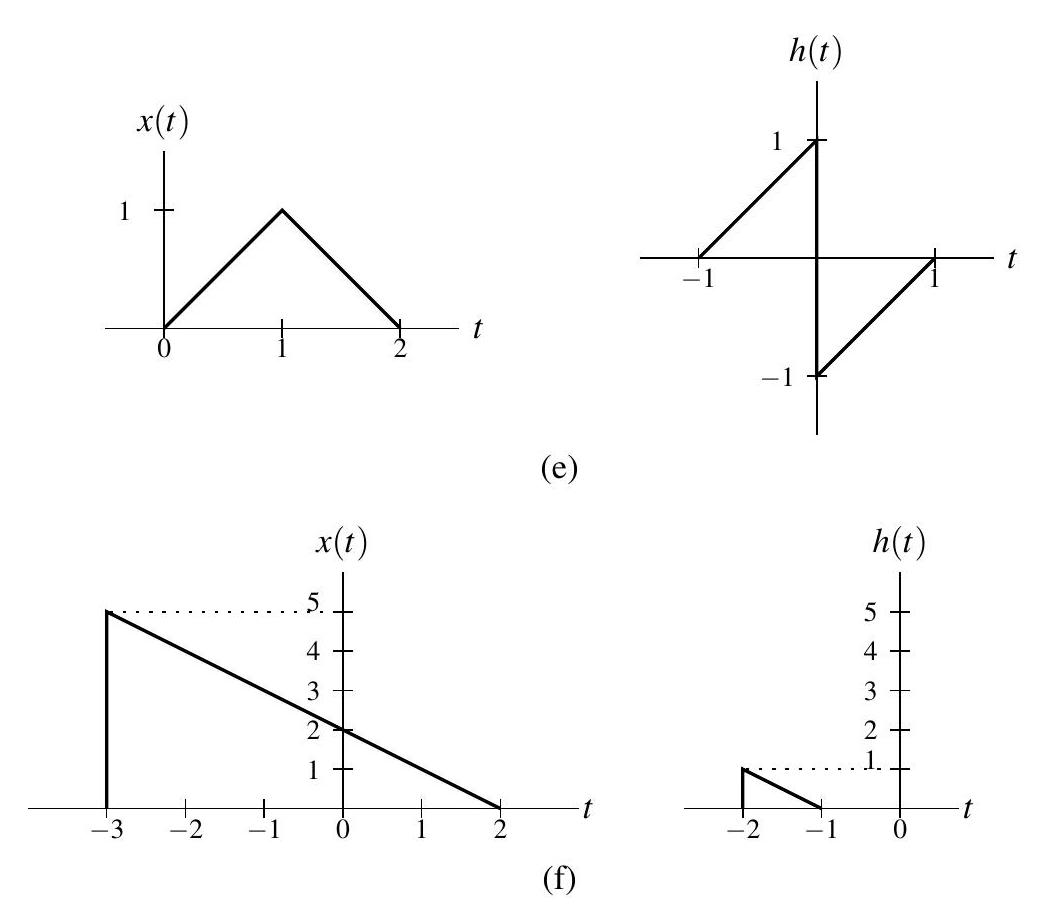
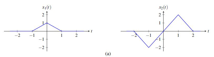
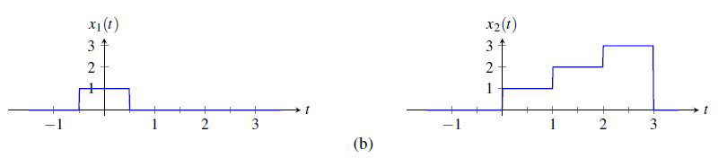
4.9 考虑一个 LTI 系统，其对函数 \(x_{1}(t)=u(t)-u(t-1)\) 的响应为 \(y_{1}\)。确定系统对图中所示输入 \(x_{2}\) 的响应 \(y_{2}\)，并用 \(y_{1}\) 表示。

4.10 考虑下图所示的系统，其中 \(\mathcal{H}\) 是 LTI 系统，\(\mathcal{G}\) 已知为 \(\mathcal{H}\) 的逆系统。设 \(y_{1}=\mathcal{H} x_{1}\)，\(y_{2}=\mathcal{H} x_{2}\)。

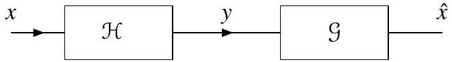
(a) 确定系统 \(\mathcal{G}\) 对输入 \(y^{\prime}(t)=a_{1} y_{1}(t)+a_{2} y_{2}(t)\) 的响应，其中 \(a_{1}\) 和 \(a_{2}\) 为复常数。
(b) 确定系统 \(\mathcal{G}\) 对输入 \(y_{1}^{\prime}(t)=y_{1}\left(t-t_{0}\right)\) 的响应，其中 \(t_{0}\) 为实常数。
(c) 利用本题前两部分的结果，判断系统 \(\mathcal{G}\) 是否是线性和/或时不变的。

4.11 求下列各方程所描述的 LTI 系统 \(\mathcal{H}\) 的冲激响应。
(a) \(\mathcal{H} x(t)=\int_{-\infty}^{t+1} x(\tau) d \tau\)；
(b) \(\mathcal{H} x(t)=\int_{-\infty}^{\infty} x(\tau+5) e^{\tau-t+1} u(t-\tau-2) d \tau\)；
(c) \(\mathcal{H} x(t)=\int_{-\infty}^{t} x(\tau) v(t-\tau) d \tau\)；
(d) \(\mathcal{H} x(t)=\int_{t-1}^{t} x(\tau) d \tau\)。

4.12 考虑下图所示的系统，其输入为 \(x\)，输出为 \(y\)。图中每个系统都是 LTI 系统，并标有其冲激响应。

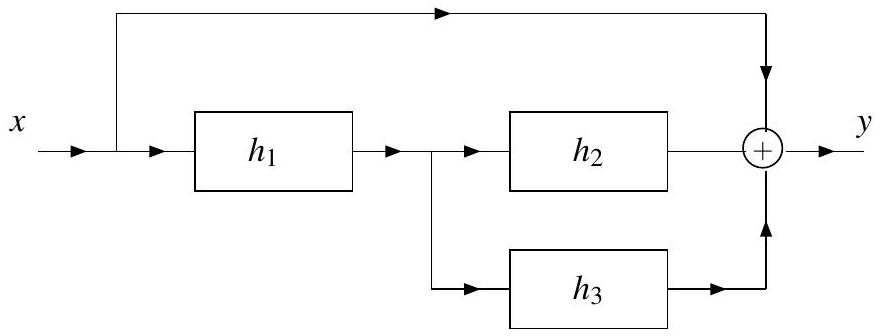
(a) 用 \(h_{1}, h_{2}, h_{3}\) 表示整体系统的冲激响应 \(h\)；
(b) 在特定情况下，确定冲激响应 \(h\)，其中

\[ h_{1}(t)=\delta(t+1), \quad h_{2}(t)=\delta(t), \quad \text { 且 } \quad h_{3}(t)=\delta(t) . \]

4.13 考虑下图所示的系统，其输入为 \(x\)，输出为 \(y\)。该系统由两个 LTI 系统串联组成，其冲激响应分别为 \(h_{1}\) 和 \(h_{2}\)。

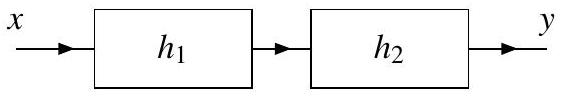
对于下列每对 \(h_{1}\) 和 \(h_{2}\)，求输入 \(x(t)=u(t)\) 时的输出 \(y\)。
(a) \(h_{1}(t)=\delta(t)\) 且 \(h_{2}(t)=\delta(t)\)；
(b) \(h_{1}(t)=\delta(t+1)\) 且 \(h_{2}(t)=\delta(t+1)\)；
(c) \(h_{1}(t)=e^{-3 t} u(t)\) 且 \(h_{2}(t)=\delta(t)\)。

4.14 判断下列各冲激响应 \(h\) 所对应的 LTI 系统是否因果和/或无记忆。
(a) \(h(t)=(t+1) u(t-1)\)；
(b) \(h(t)=2 \delta(t+1)\)；
(c) \(h(t)=\frac{\omega_{c}}{\pi} \operatorname{sinc}\left(\omega_{c} t\right)\)；
(d) \(h(t)=e^{-4 t} u(t-1)\)；
(e) \(h(t)=e^{t} u(-1-t)\)；
(f) \(h(t)=e^{-3|t|}\)；
(g) \(h(t)=3 \delta(t)\)。

4.15 判断下列各冲激响应 \(h\) 所对应的 LTI 系统是否 BIBO 稳定。
(a) \(h(t)=e^{a t} u(-t)\)，其中 \(a\) 为严格正实常数；
(b) \(h(t)=t^{-1} u(t-1)\)；
(c) \(h(t)=e^{t} u(t)\)；
(d) \(h(t)=\delta(t-10)\)；
(e) \(h(t)=\operatorname{rect}(t)\)；
(f) \(h(t)=e^{-|t|}\)。

4.16 假设我们有两个 LTI 系统，其冲激响应为

\[ h_{1}(t)=\frac{1}{2} \delta(t-1) \quad \text { 且 } \quad h_{2}(t)=2 \delta(t+1) \]

判断这两个系统是否互为逆系统。

4.17 对下列每种情况，求 LTI 系统（系统函数为 \(H\)）对输入 \(x\) 的响应 \(y\)。
(a) \(H(s)=\frac{1}{s+1}\)，适用于 \(\operatorname{Re}(s)>-1\)，输入 \(x(t)=10+4 \cos (3 t)+2 \sin (5 t)\)；
(b) \(H(s)=\frac{1}{e^{s}(s+1)}\)，适用于 \(\operatorname{Re}(s)>-1\)，输入 \(x(t)=10+2 e^{3 t}-e^{t}\)。

4.18 考虑系统 \(\mathcal{H}_{1}, \mathcal{H}_{2}, \mathcal{H}_{3}, \mathcal{H}_{4}\)，其对复指数输入 \(x(t)=e^{j 2 t}\) 的响应为

\[ \mathcal{H}_{1} x(t)=2 e^{j 2 t}, \quad \mathcal{H}_{2} x(t)=t e^{j 2 t}, \quad \mathcal{H}_{3} x(t)=e^{j 2 t+\pi / 3}, \quad \text { 且 } \quad \mathcal{H}_{4} x(t)=\cos (2 t) . \]

对每个系统，评论其是否具有 LTI 特性。

4.11.2 带答案的习题

4.101 使用图示法，计算下列每对函数 \(x\) 和 \(h\) 的卷积 \(x * h\)。（不要通过计算 \(h * x\) 再利用卷积的交换律间接求 \(x * h\)。）

(a) \(x(t)=2 \operatorname{rect}\left(t-\frac{1}{2}\right)\) 且 \(h(t)= \begin{cases}-1 & -1 \leq t<0 \\ 1 & 0 \leq t<1 \\ 0 & \text { 其他情况 }\end{cases}\)
(b) \(x(t)=u(t-1)\) 且 \(h(t)= \begin{cases}t+1 & -1 \leq t<0 \\ t-1 & 0 \leq t<1 \\ 0 & \text { 其他情况 }\end{cases}\)
(c) \(x(t)=\left\{\begin{array}{ll}t-2 & 1 \leq t<3 \\ 0 & \text { 其他情况 }\end{array}\right.\) 且 \(h(t)=\operatorname{rect}\left[\frac{1}{2}(t+2)\right]\)
(d) \(x(t)=\operatorname{rect}\left[\frac{1}{3}\left(t-\frac{3}{2}\right)\right]\) 且 \(h(t)= \begin{cases}t-1 & 1 \leq t<2 \\ 0 & \text { 其他情况 }\end{cases}\)
(e) \(x(t)=\left\{\begin{array}{ll}\frac{1}{4}(t-1)^{2} & 1 \leq t<3 \\ 0 & \text { 其他情况 }\end{array}\right.\) 且 \(h(t)= \begin{cases}t-1 & 1 \leq t<2 \\ 0 & \text { 其他情况 }\end{cases}\)
(f) \(x(t)=\left\{\begin{array}{ll}2 \cos \left(\frac{\pi}{4} t\right) & 0 \leq t<2 \\ 0 & \text { 其他情况 }\end{array}\right.\) 且 \(h(t)= \begin{cases}2-t & 1 \leq t<2 \\ 0 & \text { 其他情况 }\end{cases}\)
(g) \(x(t)=e^{-|t|}\) 且 \(h(t)=\operatorname{rect}\left[\frac{1}{2}(t-2)\right]\)
(h) \(x(t)=\left\{\begin{array}{ll}\frac{1}{2} t-\frac{1}{2} & 1 \leq t<3 \\ 0 & \text { 其他情况 }\end{array}\right.\) 且 \(h(t)= \begin{cases}-t-1 & -2 \leq t<-1 \\ 0 & \text { 其他情况 }\end{cases}\)
(i) \(x(t)=e^{-|t|}\) 且 \(h(t)=\operatorname{tri}\left[\frac{1}{2}(t-3)\right]\)
(j) \(x(t)=\left\{\begin{array}{ll}\frac{1}{4} t-\frac{1}{4} & 1 \leq t<5 \\ 0 & \text { 其他情况 }\end{array}\right.\) 且 \(h(t)= \begin{cases}\frac{3}{2}-\frac{1}{2} t & 1 \leq t<3 \\ 0 & \text { 其他情况 }\end{cases}\)
(k) \(x(t)=\operatorname{rect}\left(\frac{1}{20} t\right)\) 且 \(h(t)= \begin{cases}t-1 & 1 \leq t<2 \\ 0 & \text { 其他情况 }\end{cases}\)
(l) \(x(t)=\left\{\begin{array}{ll}1-\frac{1}{100} t & 0 \leq t<100 \\ 0 & \text { 其他情况 }\end{array}\right.\) 且 \(h(t)=e^{-t} u(t-1)\)
(m) \(x(t)=\operatorname{rect}\left(\frac{1}{20} t\right)\) 且 \(h(t)= \begin{cases}1-(t-2)^{2} & 1 \leq t<3 \\ 0 & \text { 其他情况 }\end{cases}\)
(n) \(x(t)=e^{-t} u(t)\) 且 \(h(t)=e^{-3 t} u(t-2)\)
(o) \(x(t)=e^{-|t|}\) 且 \(h(t)=\operatorname{rect}\left(t-\frac{3}{2}\right)\)
(p) \(x(t)=e^{-2 t} u(t)\) 且 \(h(t)=\operatorname{rect}\left(t-\frac{5}{2}\right)\)
(q) \(x(t)=u(t-1)\) 且 \(h(t)= \begin{cases}\sin [\pi(t-1)] & 1 \leq t<2 \\ 0 & \text { 其他情况 }\end{cases}\)
(r) \(x(t)=u(t)\) 且 \(h(t)=\operatorname{rect}\left(\frac{1}{4}[t-4]\right)\)
(s) \(x(t)=e^{-t} u(t)\) 且 \(h(t)=e^{2-2 t} u(t-1)\)
(t) \(x(t)=e^{-3 t} u(t)\) 且 \(h(t)=u(t+1)\)
(u) \(x(t)=\left\{\begin{array}{ll}2-t & 1 \leq t<2 \\ 0 & \text { 其他情况 }\end{array}\right.\) 且 \(h(t)= \begin{cases}-t-2 & -3 \leq t<-2 \\ 0 & \text { 其他情况 }\end{cases}\) 简答

(a) \(x * h(t)= \begin{cases}\int_{0}^{t+1}-2 \, d \tau & -1 \leq t<0 \\ \int_{0}^{t} 2 \, d \tau+\int_{t}^{1}-2 \, d \tau & 0 \leq t<1 \\ \int_{t-1}^{1} 2 \, d \tau & 1 \leq t<2 \\ 0 & \text { 其他情况 }\end{cases}\)

(b) \(x * h(t)= \begin{cases}\int_{1}^{t+1}(-\tau+t+1) \, d \tau & 0 \leq t<1 \\ \int_{1}^{t}(-\tau+t-1) \, d \tau+\int_{t}^{t+1}(-\tau+t+1) \, d \tau & 1 \leq t<2 \\ \int_{t-1}^{t}(-\tau+t-1) \, d \tau+\int_{t}^{t+1}(-\tau+t+1) \, d \tau & t \geq 2 \\ 0 & \text { 其他情况 }\end{cases}\)

(c) \(x * h(t)= \begin{cases}\int_{1}^{t+3}(\tau-2) \, d \tau & -2 \leq t<0 \\ \int_{t+1}^{3}(\tau-2) \, d \tau & 0 \leq t<2 \\ 0 & \text { 其他情况 }\end{cases}\)

(d) \(x * h(t)= \begin{cases}\int_{0}^{t-1}(t-\tau-1) \, d \tau & 1 \leq t<2 \\ \int_{t-2}^{t-1}(t-\tau-1) \, d \tau & 2 \leq t<4 \\ \int_{t-2}^{3}(t-\tau-1) \, d \tau & 4 \leq t<5 \\ 0 & \text { 其他情况 }\end{cases}\)

(e) \(x * h(t)= \begin{cases}\int_{1}^{t-1} \frac{1}{4}(\tau-1)^{2}(t-\tau-1) \, d \tau & 2 \leq t<3 \\ \int_{t-2}^{t-1} \frac{1}{4}(\tau-1)^{2}(t-\tau-1) \, d \tau & 3 \leq t<4 \\ \int_{t-2}^{3} \frac{1}{4}(\tau-1)^{2}(t-\tau-1) \, d \tau & 4 \leq t<5 \\ 0 & \text { 其他情况 }\end{cases}\)

(f) \(x * h(t)= \begin{cases}\int_{0}^{t-1} 2 \cos \left(\frac{\pi}{4} \tau\right)(\tau-t+2) \, d \tau & 1 \leq t<2 \\ \int_{t-2}^{t-1} 2 \cos \left(\frac{\pi}{4} \tau\right)(\tau-t+2) \, d \tau & 2 \leq t<3 \\ \int_{t-2}^{2} 2 \cos \left(\frac{\pi}{4} \tau\right)(\tau-t+2) \, d \tau & 3 \leq t<4 \\ 0 & \text { 其他情况 }\end{cases}\)

(g) \(x * h(t)= \begin{cases}\int_{t-3}^{t-1} e^{\tau} \, d \tau & t<1 \\ \int_{t-3}^{0} e^{\tau} \, d \tau+\int_{0}^{t-1} e^{-\tau} \, d \tau & 1 \leq t<3 \\ \int_{t-3}^{t-1} e^{-\tau} \, d \tau & t \geq 3 \end{cases}\)

(h) \(x * h(t)= \begin{cases}\int_{1}^{t+2}\left(\frac{1}{2} \tau-\frac{1}{2}\right)(\tau-t-1) \, d \tau & -1 \leq t<0 \\ \int_{t+1}^{t+2}\left(\frac{1}{2} \tau-\frac{1}{2}\right)(\tau-t-1) \, d \tau & 0 \leq t<1 \\ \int_{t+1}^{3}\left(\frac{1}{2} \tau-\frac{1}{2}\right)(\tau-t-1) \, d \tau & 1 \leq t<2 \\ 0 & \text { 其他情况 }\end{cases}\)

(i) \(x * h(t)= \begin{cases}\int_{t-4}^{t-3} e^{\tau}(\tau-t+4) \, d \tau+\int_{t-3}^{t-2} e^{\tau}(t-\tau-2) \, d \tau & t<2 \\ \int_{t-4}^{t-3} e^{\tau}(\tau-t+4) \, d \tau+\int_{t-3}^{0} e^{\tau}(t-\tau-2) \, d \tau+\int_{0}^{t-2} e^{-\tau}(t-\tau-2) \, d \tau & 2 \leq t<3 \\ \int_{t-4}^{0} e^{\tau}(\tau-t+4) \, d \tau+\int_{0}^{t-3} e^{-\tau}(t-\tau+4) \, d \tau+\int_{t-3}^{t-2} e^{-\tau}(t-\tau-2) \, d \tau & 3 \leq t<4 \\ \int_{t-4}^{t-3} e^{-\tau}(\tau-t+4) \, d \tau+\int_{t-3}^{t-2} e^{-\tau}(t-\tau-2) \, d \tau & t \geq 4 \end{cases}\)

(j) \(x * h(t)= \begin{cases}\int_{1}^{t-1}\left(\frac{1}{4} \tau-\frac{1}{4}\right)\left(\frac{1}{2} \tau-\frac{1}{2} t+\frac{3}{2}\right) \, d \tau & 2 \leq t<4 \\ \int_{t-3}^{t-1}\left(\frac{1}{4} \tau-\frac{1}{4}\right)\left(\frac{1}{2} \tau-\frac{1}{2} t+\frac{3}{2}\right) \, d \tau & 4 \leq t<6 \\ \int_{t-3}^{5}\left(\frac{1}{4} \tau-\frac{1}{4}\right)\left(\frac{1}{2} \tau-\frac{1}{2} t+\frac{3}{2}\right) \, d \tau & 6 \leq t<8 \\ 0 & \text { 其他情况 }\end{cases}\)

(k) \(x * h(t)= \begin{cases}\int_{-10}^{t-1}(t-\tau-1) \, d \tau & -9 \leq t<-8 \\ \int_{t-2}^{t-1}(t-\tau-1) \, d \tau & -8 \leq t<11 \\ \int_{t-2}^{10}(t-\tau-1) \, d \tau & 11 \leq t<12 \\ 0 & \text { 其他情况 }\end{cases}\)

(l) \(x * h(t)= \begin{cases}0 & t<1 \\ \int_{0}^{t-1}\left(1-\frac{1}{100} \tau\right) e^{\tau-t} \, d \tau & 1 \leq t<101 \\ \int_{0}^{100}\left(1-\frac{1}{100} \tau\right) e^{\tau-t} \, d \tau & t \geq 101 \end{cases}\)

(m) \(x * h(t)= \begin{cases}\int_{-10}^{t-1}\left[1-(t-\tau-2)^{2}\right] \, d \tau & -9 \leq t<-7 \\ \int_{t-3}^{t-1}\left[1-(t-\tau-2)^{2}\right] \, d \tau & -7 \leq t<11 \\ \int_{t-3}^{10}\left[1-(t-\tau-2)^{2}\right] \, d \tau & 11 \leq t<13 \\ 0 & \text { 其他情况 }\end{cases}\)

(n) \(x * h(t)= \begin{cases}\int_{0}^{t-2} e^{-\tau} e^{3 \tau-3 t} \, d \tau & t \geq 2 \\ 0 & \text { 其他情况 }\end{cases}\)

(o) \(x * h(t)= \begin{cases}\int_{t-2}^{t-1} e^{\tau} \, d \tau & t<1 \\ \int_{t-2}^{0} e^{\tau} \, d \tau+\int_{0}^{t-1} e^{-\tau} \, d \tau & 1 \leq t<2 \\ \int_{t-2}^{t-1} e^{-\tau} \, d \tau & t \geq 2 \end{cases}\)

(p) \(x * h(t)= \begin{cases}0 & t<2 \\ \int_{0}^{t-2} e^{-2 \tau} \, d \tau & 2 \leq t<3 \\ \int_{t-3}^{t-2} e^{-2 \tau} \, d \tau & t \geq 3 \end{cases}\)

(q) \(x * h(t)= \begin{cases}0 & t<2 \\ \int_{1}^{t-1} \sin (\pi t-\pi \tau-\pi) \, d \tau & 2 \leq t<3 \\ \int_{t-2}^{t-1} \sin (\pi t-\pi \tau-\pi) \, d \tau & t \geq 3 \end{cases}\)

(r) \(x * h(t)= \begin{cases}0 & t<2 \\ \int_{0}^{t-2} 1 \, d \tau & 2 \leq t<6 \\ \int_{t-6}^{t-2} 1 \, d \tau & t \geq 6 \end{cases}\)

(s) \(x * h(t)= \begin{cases}\int_{0}^{t-1} e^{\tau-2 t+2} \, d \tau & t \geq 1 \\ 0 & \text { 其他情况 }\end{cases}\)

(t) \(x * h(t)= \begin{cases}\int_{0}^{t+1} e^{-3 \tau} \, d \tau & t \geq -1 \\ 0 & \text { 其他情况 }\end{cases}\)

(u) \(x * h(t)= \begin{cases}\frac{1}{6} t^{3}-t-\frac{2}{3} & -2 \leq t<-1 \\ -\frac{1}{6} t^{3} & -1 \leq t<0 \\ 0 & \text { 其他情况 }\end{cases}\) 4.102 使用图解法，计算下列每对函数 \(x\) 和 \(h\) 的卷积 \(x * h\)。
(a) \(x(t)=\operatorname{rect}\left(\frac{1}{2 a} t\right)\)，\(h(t)=\operatorname{rect}\left(\frac{1}{2 a} t\right)\)；
(b) \(x(t)=\operatorname{rect}\left(\frac{1}{a} t\right)\)，\(h(t)=\operatorname{rect}\left(\frac{1}{a} t\right)\)。

简答
(a) \(x * h(t)=2 a \operatorname{tri}\left(\frac{1}{4 a} t\right)\)；
(b) \(x * h(t)=a \operatorname{tri}\left(\frac{1}{2 a} t\right)\)。

4.103 设 \(\mathcal{H}\) 表示对应于 LTI 系统的算子，\(\mathcal{S}_{t_{0}}\) 表示平移算子（即 \(\mathcal{S}_{t_{0}} x(t)=x(t-t_{0})\) 对所有 \(t\) 成立）。设 \(x_{1}, x_{2}, \ldots, x_{n}, y_{1}, y_{2}, \ldots, y_{n}, x\) 和 \(y\) 为函数，满足 \(y_{k}=\mathcal{H} x_{k}\)，\(y=\mathcal{H} x\)。求 \(y\) 用 \(y_{1}, y_{2}, \ldots, y_{n}\) 表示。

简答
(a) \(y=\pi y_{1}\)；
(b) \(y=y_{1}+y_{2}\)；
(c) \(y=j y_{1}+\pi y_{2}\)；
(d) \(y=\mathcal{S}_{42} y_{1}\)；
(e) \(y=3 \mathcal{S}_{-2} y_{1}\)；
(f) \(y=2 \mathcal{S}_{3} y_{1}+j \pi \mathcal{S}_{-5} y_{2}\)；
(g) \(y=\sum_{k=1}^{10} k \mathcal{S}_{k} y_{k}\)。

4.104 设 \(\mathcal{H}\) 表示对应于 LTI 系统的算子，\(x_{1}, x_{2}, y_{1}, y_{2}\) 为函数，满足 \(y_{1}=\mathcal{H} x_{1}\)，\(y_{2}=\mathcal{H} x_{2}\)。对于下列每对 \(x_{1}\) 和 \(x_{2}\)，求 \(y_{2}\) 用 \(y_{1}\) 表示。

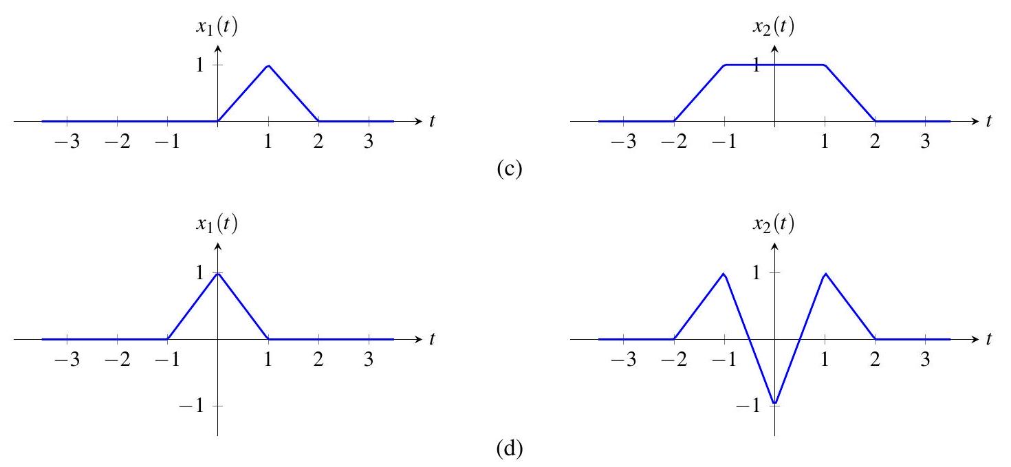
简答
(a) \(y_{2}(t)=-2 y_{1}(t+1)+2 y_{1}(t-1)\)；
(b) \(y_{2}(t)=y_{1}\left(t-\frac{1}{2}\right)+2 y_{1}\left(t-\frac{3}{2}\right)+3 y_{1}\left(t-\frac{5}{2}\right)\)；
(c) \(y_{2}(t)=y_{1}(t+2)+y_{1}(t+1)+y_{1}(t)\)；
(d) \(y_{2}(t)=y_{1}(t+1)-y_{1}(t)+y_{1}(t-1)\)。

4.105 设 \(\mathscr{H}_{k}\)（\(k\) 为整数）表示具有冲激响应 \(h_{k}\) 的 LTI 系统算子。求由下列方程表征的系统 \(\mathcal{H}\) 的冲激响应 \(h\) 用 \(h_{k}\) 表示。

简答
(a) \(h=2(h_{1}-h_{2})\)；
(b) \(h=\frac{2}{3} h_{1} * h_{2}\)；
(c) \(h=5 \delta-3 h_{1}+\frac{2}{5} h_{2}\)；
(d) \(h=h_{1} * (h_{2} * h_{3}+h_{3}+\delta)\)；
(e) \(h=2 (h_{1}+h_{2}) * (h_{1}+h_{2})\)。

4.106 求由下列方程表征的 LTI 系统 \(\mathcal{H}\) 的冲激响应。
(a) \(\mathcal{H} x(t)=\int_{t}^{\infty} x(\tau) d \tau\)；
(b) \(\mathcal{H} x(t)=\int_{-\infty}^{\infty} e^{-|\tau|} x(t-\tau) d \tau\)；
(c) \(\mathcal{H} x(t)=\int_{t-5}^{t-4} x(\tau) d \tau\)；
(d) \(\mathcal{H} x(t)=x(t)+x(t-1)\)。

简答
(a) \(h(t)=u(-t)\)；
(b) \(h(t)=e^{-|t|}\)；
(c) \(h(t)=u(t-4)-u(t-5)\)；
(d) \(h(t)=\delta(t)+\delta(t-1)\)。

4.107 判定下列冲激响应 \(h\) 的 LTI 系统是否因果和/或无记忆。
(a) \(h(t)=u(t+1)-u(t-1)\)；
(b) \(h(t)=e^{-5 t} u(t-1)\)；
(c) \(h(t)=(t^{2}-1) \sin(t) \delta(t+1)\)；
(d) \(h(t)=\pi \delta(t+42)\)；
(e) \(h(t)=(t^{2}+4)[u(t+5)-u(t+3)]\)；
(f) \(h(t)=\cos(t)\delta(t+\pi/2)+5\delta(t)\)。

简答
(a) 有记忆，不因果；
(b) 有记忆，因果；
(c) 无记忆，因果；
(d) 有记忆，不因果；
(e) 有记忆，不因果；
(f) 无记忆，因果。

4.108 判定下列冲激响应 \(h\) 的 LTI 系统是否 BIBO 稳定。
(a) \(h(t)=u(t-1)-u(t-2)\)；
(b) \(h(t)=e^{-2 t^{2}}\)（提示：\(\int_{-\infty}^{\infty} e^{-t^{2}} dt=\sqrt{\pi}\)）；
(c) \(h(t)=t^{-2} u(-t-1)\)；
(d) \(h(t)=e^{-t} \sin(t) u(t)\)；
(e) \(h(t)=e^{-t} u(-t)\)；
(f) \(h(t)=t e^{-3 t} u(t-1)\) [提示：参见 (F.1)] ；
(g) \(h(t)=t e^{-2 t} u(1-t)\)[提示：参见 (F.1)]。

简答
(a) BIBO 稳定 \(\left(\int_{-\infty}^{\infty}|h(t)| dt=1\right)\)；
(b) BIBO 稳定 \(\left(\int_{-\infty}^{\infty}|h(t)| dt=\sqrt{\pi/2}\right)\)；
(c) BIBO 稳定 \(\left(\int_{-\infty}^{\infty}|h(t)| dt=1\right)\)；
(d) BIBO 稳定 \(\left(\int_{-\infty}^{\infty}|h(t)| dt \le 1\right)\)；
(e) 不 BIBO 稳定；
(f) BIBO 稳定 \(\left(\int_{-\infty}^{\infty}|h(t)| dt=4/(9 e^{3})\right)\)；
(g) 不 BIBO 稳定。

4.109 求下列系统函数 \(H\) 的 LTI 系统对输入 \(x\) 的输出 \(y\)。
(a) \(H(s)=\frac{1}{(s+1)(s+2)}\)，\(x(t)=1+\frac{1}{2} e^{-t/2}+\frac{1}{3} e^{-t/3}\)；
(b) \(H(s)=s\)，\(x(t)=1+2 e^{-t/2}+3 e^{-t/3}\)；
(c) \(H(s)=\frac{1}{s+1}\)，\(x(t)=2 \cos(t)\)；
(d) \(H(s)=s e^{-s}\)，\(x(t)=4 \cos(t)+2 \sin(3 t)\)；
(e) \(H(s)=\frac{1}{e^{s}(s+4)}\)，\(x(t)=11+7 e^{-2 t}+5 e^{-3 t}\)；
(f) \(H(s)=s^{2}\)，\(x(t)=7+e^{-5 t}+4 \cos(3 t)\)。

简答
(a) \(y(t)=\frac{1}{2}+\frac{2}{3} e^{-t/2}+\frac{3}{10} e^{-t/3}\)；
(b) \(y(t)=-e^{-t/2}-e^{-t/3}\)；
(c) \(y(t)=\sqrt{2} \cos(t-\pi/4)\)；
(d) \(y(t)=6 \cos(3 t-3)-4 \sin(t-1)\)；
(e) \(y(t)=\frac{11}{4}+ \frac{7}{2} e^{2(1-t)} + 5 e^{3(1-t)}\)；
(f) \(y(t)=25 e^{-5 t}-36 \cos(3 t)\)。

4.11.3 MATLAB 练习

当前暂无 MATLAB 练习。